tensorflow神经网络拟合非线性函数
内容导读
互联网集市收集整理的这篇技术教程文章主要介绍了tensorflow神经网络拟合非线性函数,小编现在分享给大家,供广大互联网技能从业者学习和参考。文章包含2411字,纯文字阅读大概需要4分钟。
内容图文

本实验通过建立一个含有两个隐含层的BP神经网络,拟合具有二次函数非线性关系的方程,并通过可视化展现学习到的拟合曲线,同时随机给定输入值,输出预测值,最后给出一些关键的提示。
源代码如下:
            #
             -*- coding: utf-8 -*-
            import
             tensorflow as tf

            import
             numpy as np

            import
             matplotlib.pyplot as plt

plotdata = { "batchsize":[], "loss":[] }
def moving_average(a, w=11):
    if len(a) < w:
        return a[:]
    return [val if idx < w else sum(a[(idx-w):idx])/w for idx, val in enumerate(a)]

#生成模拟数据,二次函数关系
train_X = np.linspace(-1, 1, 100)[:, np.newaxis]
train_Y = train_X*train_X + 5 * train_X + np.random.randn(*train_X.shape) * 0.3

#子图1显示模拟数据点
plt.figure(12)
plt.subplot(221)
plt.plot(train_X, train_Y, ‘ro‘, label=‘Original data‘)
plt.legend()

# 创建模型
# 占位符
X = tf.placeholder("float",[None,1])
Y = tf.placeholder("float",[None,1])
# 模型参数
W1 = tf.Variable(tf.random_normal([1,10]), name="weight")
b1 = tf.Variable(tf.zeros([1,10]), name="bias")
W2 = tf.Variable(tf.random_normal([10,6]), name="weight")
b2 = tf.Variable(tf.zeros([1,6]), name="bias")
W3 = tf.Variable(tf.random_normal([6,1]), name="weight")
b3 = tf.Variable(tf.zeros([1]), name="bias")

# 前向结构
z1 = tf.matmul(X, W1) + b1
z2 = tf.nn.relu(z1)
z3 = tf.matmul(z2, W2) + b2
z4 = tf.nn.relu(z3)
z5 = tf.matmul(z4, W3) + b3

#反向优化
cost =tf.reduce_mean( tf.square(Y - z5))
learning_rate = 0.01
optimizer = tf.train.GradientDescentOptimizer(learning_rate).minimize(cost) #Gradient descent# 初始化变量
init = tf.global_variables_initializer()
# 训练参数
training_epochs = 5000
display_step = 2

# 启动sessionwith tf.Session() as sess:
    sess.run(init)
    for epoch in range(training_epochs+1):
        sess.run(optimizer, feed_dict={X: train_X, Y: train_Y})

        #显示训练中的详细信息if epoch % display_step == 0:
            loss = sess.run(cost, feed_dict={X: train_X, Y:train_Y})
            print ("Epoch:", epoch, "cost=", loss)
            ifnot (loss == "NA" ):
                plotdata["batchsize"].append(epoch)
                plotdata["loss"].append(loss)
    print (" Finish")

    #图形显示
    plt.subplot(222)
    plt.plot(train_X, train_Y, ‘ro‘, label=‘Original data‘)
    plt.plot(train_X, sess.run(z5, feed_dict={X: train_X}), label=‘Fitted line‘)
    plt.legend()
    plotdata["avgloss"] = moving_average(plotdata["loss"])

    plt.subplot(212)
    plt.plot(plotdata["batchsize"], plotdata["avgloss"], ‘b--‘)
    plt.xlabel(‘Minibatch number‘)
    plt.ylabel(‘Loss‘)
    plt.title(‘Minibatch run vs Training loss‘)
    plt.show()
    #预测结果
    a=[[0.2],[0.3]]
    print ("x=[[0.2],[0.3]],z5=", sess.run(z5, feed_dict={X: a}))
运行结果如下:
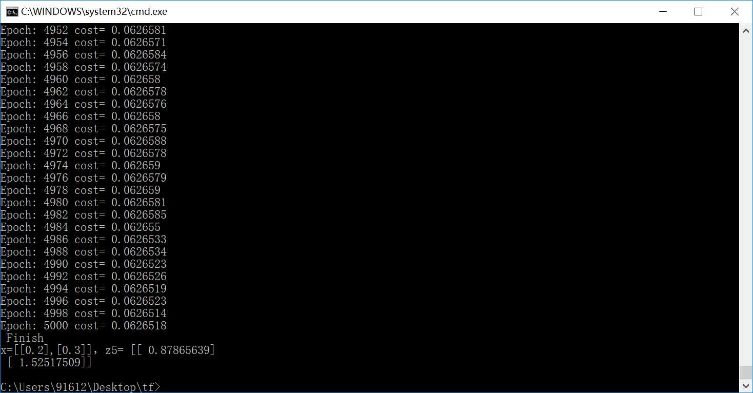
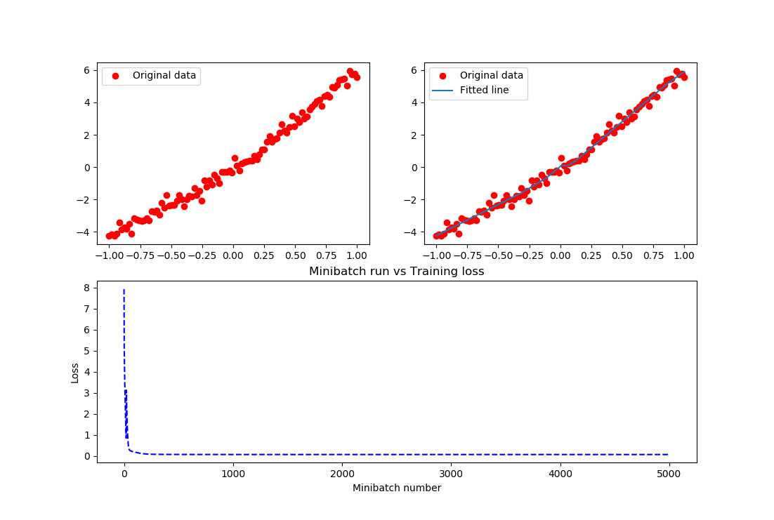
结果实在是太棒了,把这个关系拟合的非常好。
原文:https://www.cnblogs.com/cvtoEyes/p/9063291.html
内容总结
以上是互联网集市为您收集整理的tensorflow神经网络拟合非线性函数全部内容,希望文章能够帮你解决tensorflow神经网络拟合非线性函数所遇到的程序开发问题。 如果觉得互联网集市技术教程内容还不错,欢迎将互联网集市网站推荐给程序员好友。
内容备注
版权声明:本文内容由互联网用户自发贡献,该文观点与技术仅代表作者本人。本站仅提供信息存储空间服务,不拥有所有权,不承担相关法律责任。如发现本站有涉嫌侵权/违法违规的内容, 请发送邮件至 gblab@vip.qq.com 举报,一经查实,本站将立刻删除。
内容手机端
扫描二维码推送至手机访问。
来源:【匿名】