首页 / PYTHON / 用卡尔曼滤波器跟踪导弹（给出matlab和python的仿真代码）

用卡尔曼滤波器跟踪导弹（给出matlab和python的仿真代码）

内容导读

互联网集市收集整理的这篇技术教程文章主要介绍了用卡尔曼滤波器跟踪导弹（给出matlab和python的仿真代码），小编现在分享给大家，供广大互联网技能从业者学习和参考。文章包含7268字，纯文字阅读大概需要11分钟。

内容图文

题目

巡航导弹沿直线飞向目标，目标处设有一监视雷达，雷达对导弹的距离进行观测。
假设：（1）导弹初始距离 100 k m 100km 100km，速度约为 300 m / s 300m/s 300m/s，基本匀速飞行，但受空气扰动影响，扰动加速度为零均值白噪声，方差强度 q = 0.05 m 2 / s 3 q=0.05m^2/s^3 q=0.05m2/s3 ；（2）雷达观测频率 2 H z 2Hz 2Hz，观测误差为零均值白噪声，均方差为 50 m 50m 50m。
试使用卡尔曼滤波（Kalman filter）完成导弹的轨迹跟踪。

matlab仿真代码

%%%%%%%%%%%%%%%%%%%%%%%%%%%%%%%%%%%%%%%%%%%%%%%%%%%%%%%%%%%%%%%%%%%%%%%%%%
% 功能描述：导弹运动Kalman滤波程序
%%%%%%%%%%%%%%%%%%%%%%%%%%%%%%%%%%%%%%%%%%%%%%%%%%%%%%%%%%%%%%%%%%%%%%%%%%
clear;clc;close all;
%% 01 初始化参数
T = 300;

Ts = 1/2;               % 采样时间
Q = 0.05*Ts;            % 过程噪声 
R = 50/Ts;              % 量测噪声
W = sqrt(Q)*randn(1,T);
V = sqrt(R)*randn(1,T);
P0 = diag([10^2,1^2]);  

% 系统矩阵
Phi = [1,-Ts;0,1];
H = [1,0];
Tau = [0.5*Ts^2;Ts];

% 初始化
nS = 2; nZ = 1;
xState = zeros(nS,T);
zMea = zeros(nZ,T);
xKF = zeros(nS,T);
xKF_pre = zeros(nS,T);
xState(:,1) = [100000;300];
zMea(:,1) = H*xState(:,1);
xKF(:,1) = xState(:,1);
%% 02 用模型模拟真实状态
for t = 2:T
    xState(:,t) = Phi*xState(:,t-1) + Tau*W(:,t);
    zMea(:,t) = H*xState(:,t) + V(t);
end
%% 03 Kalman滤波
for t = 2:T
    xKF_pre(:,t) = Phi*xKF(:,t-1);
    P_pre = Phi*P0*Phi' + Tau*Q*Tau';
    K = P_pre*H'*pinv(H*P_pre*H'+R);
    xKF(:,t) = xKF_pre(:,t) + K*(zMea(:,t)-H*xKF_pre(:,t));
    P0 = (eye(2)-K*H)*P_pre;
end
%% 04 画图
tPlot = 1:T;
FigWin1=figure('position',[300 400 550 450],'Color',[0.8 0.8 0.8],...
   'Name','01-量测距离误差与估计距离误差的比较','NumberTitle','off');hold on;box on;
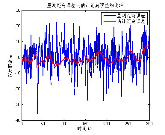
plot(tPlot,xState(1,:)-zMea(1,:),'-b','LineWidth',1.5);hold on;
plot(tPlot,xState(1,:)-xKF(1,:),'-r','LineWidth',1.5);hold on;
xlabel('时间 t/s');ylabel('误差距离 m');
legend('量测距离误差','估计距离误差');
title('量测距离误差与估计距离误差的比较');

FigWin2=figure('position',[850 400 550 450],'Color',[0.8 0.8 0.8],...
   'Name','02-真实速度与估计速度的比较','NumberTitle','off');hold on;box on;
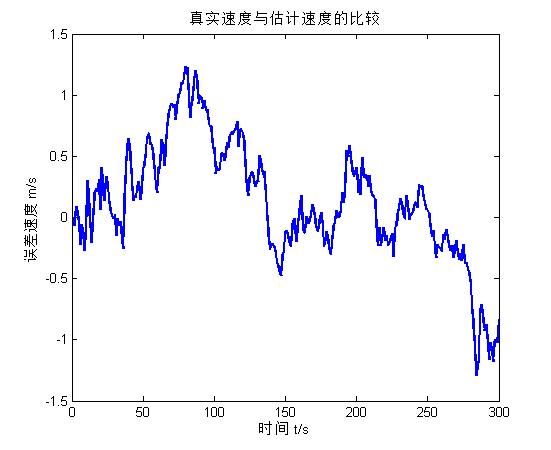
plot(tPlot,xState(2,:)-xKF(2,:),'-b','LineWidth',1.5);hold on;
xlabel('时间 t/s');ylabel('误差速度 m/s');
title('真实速度与估计速度的比较');

FigWin3=figure('position',[300 200 550 450],'Color',[0.8 0.8 0.8],...
   'Name','03-导弹真实轨迹与雷达量测','NumberTitle','off');hold on;box on;
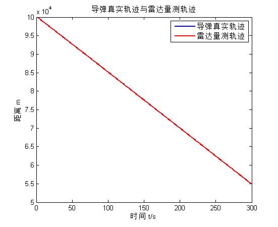
plot(tPlot,xState(1,:),'-b','LineWidth',1.5);hold on;
plot(tPlot,zMea(1,:),'-r','LineWidth',1.5);hold on;
xlabel('时间 t/s');ylabel('距离 m');
legend('导弹真实轨迹','雷达量测轨迹');
title('导弹真实轨迹与雷达量测轨迹');

FigWin4=figure('position',[850 200 550 450],'Color',[0.8 0.8 0.8],...
   'Name','04-估计距离与估计速度','NumberTitle','off');hold on;box on;
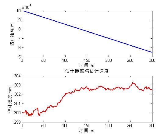
subplot(211);
plot(tPlot,xKF(1,:),'-b','LineWidth',1.5);hold on;
xlabel('时间 t/s');ylabel('估计距离 m');
subplot(212);
plot(tPlot,xKF(2,:),'-r','LineWidth',1.5);hold on;
xlabel('时间 t/s');ylabel('估计速度 m/s');
title('估计距离与估计速度');

仿真结果图如下所示。
用卡尔曼滤波器跟踪导弹（给出matlab和python的仿真代码） - 文章图片

python仿真代码

"""
#-------------------------------------------------------------------#
#                     Li Lingwei's Python Code                      #     
#-------------------------------------------------------------------#
#                                                                   #
#                   @Project Name : Matlab to python                #
#                   @File Name    : Kamlan.py                       #
#                   @Programmer   : Li Lingwei                      #
#                   @Start Date   : 2021/4/18                       #
#                   @Last Update  : 2021/4/26                       #
#-------------------------------------------------------------------#
# Function:                                                         #
#                                                                   #
#-------------------------------------------------------------------#
"""
import numpy as np
import pylab as plt

"""01 初始化参数"""
T = 300

Ts = 1 / 2  # 采样时间
Q = 0.05 * Ts  # 过程噪声
R = 50 / Ts  # 量测噪声
W = np.sqrt(Q) * np.random.randn(1, T)
V = np.sqrt(R) * np.random.randn(1, T)
P0 = np.diag([10 ** 2, 1 ** 2])

# 系统矩阵
Phi = np.mat([[1, -Ts],
              [0, 1]])
H = np.mat([1, 0])
Tau = np.mat([[0.5 * (Ts ** 2)],
              [Ts]])

# 初始化
nS = 2
nZ = 1
xState = np.zeros([nS, T])
xState = np.mat(xState)
zMea = np.zeros([nZ, T])
zMea = np.mat(zMea)
xKF = np.zeros([nS, T])
xKF = np.mat(xKF)
xKF_pre = np.zeros([nS, T])
xKF_pre = np.mat(xKF_pre)
xState[:, 0] = [[100000], [300]]
xKF[:, 0] = xState[:, 0]
zMea[:, 0] = H * xState[:, 0]

"""02 用模型模拟真实状态"""
for t in range(1, T):
    xState[:, t] = Phi * xState[:, t - 1] + Tau * W[:, t]
    zMea[:, t] = H * xState[:, t] + V[:, t]

"""03 Kalman滤波"""
for t in range(1, T):
    xKF_pre[:, t] = Phi * xKF[:, t - 1]
    P_pre = Phi * P0 * Phi.T + Tau * Q * Tau.T
    K = P_pre * H.T * np.linalg.pinv(H * P_pre * H.T + R)
    xKF[:, t] = xKF_pre[:, t] + K * (zMea[:, t] - H * xKF_pre[:, t])
    P0 = (np.identity(nS) - K * H) * P_pre

"""04 画图"""
font = {'family': 'Times New Roman',
        'weight': 'normal',
        'size': 10}
fontTitle = {'family': 'Times New Roman',
             'weight': 'normal',
             'size': 12}
# 变成数组才可以画图
t = [t for t in range(1, T+1)]
xStatePlot = xState.getA()
xKFPlot = xKF.getA()
zMeaPlot = zMea.getA()

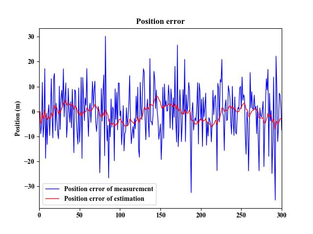
# 01 量测距离误差与估计距离误差的比较
plt.figure(1)
plt.plot(t, xStatePlot[0, :]-zMeaPlot[0, :], 'b', linewidth=1, label='Position error of measurement')
plt.plot(t, xStatePlot[0, :]-xKFPlot[0, :], 'r', linewidth=1, label='Position error of estimation')
plt.title('Position error', fontdict=fontTitle)
plt.ylabel('Position (m)', fontdict=font)
plt.tick_params(pad=3)
plt.yticks(fontproperties='Times New Roman', size=10)
plt.xticks(fontproperties='Times New Roman', size=10)
plt.xlim(0, T)
plt.legend(prop=font)

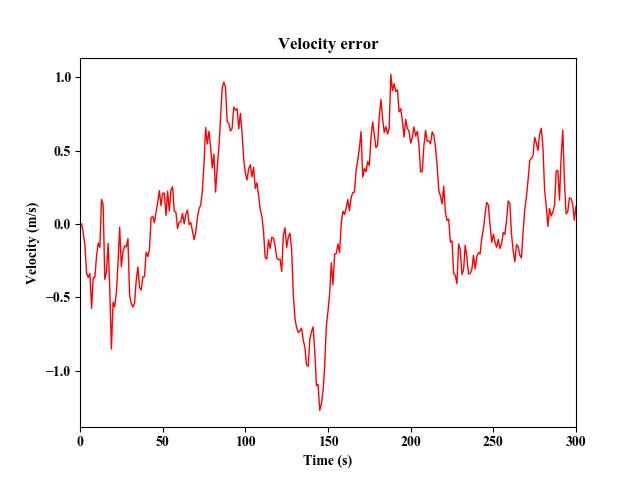
# 02 真实速度与估计速度的比较
plt.figure(2)
plt.plot(t, xStatePlot[1, :]-xKFPlot[1, :], 'r', linewidth=1)
plt.title('Velocity error', fontdict=fontTitle)
plt.xlabel('Time (s)', fontdict=font), plt.ylabel('Velocity (m/s)', fontdict=font)
plt.tick_params(pad=3)
plt.yticks(fontproperties='Times New Roman', size=10)
plt.xticks(fontproperties='Times New Roman', size=10)
plt.xlim(0, T)

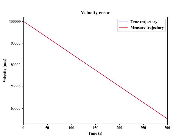
# 03 导弹真实轨迹与雷达量测
plt.figure(3)
plt.plot(t, xStatePlot[0, :], 'b', linewidth=1, label='True trajectory')
plt.plot(t, zMeaPlot[0, :], 'r', linewidth=1, label='Measure trajectory')
plt.title('Velocity error', fontdict=fontTitle)
plt.xlabel('Time (s)', fontdict=font), plt.ylabel('Velocity (m/s)', fontdict=font)
plt.tick_params(pad=3)
plt.yticks(fontproperties='Times New Roman', size=10)
plt.xticks(fontproperties='Times New Roman', size=10)
plt.xlim(0, T)
plt.legend(prop={'family': 'Times New Roman', 'size': 10})

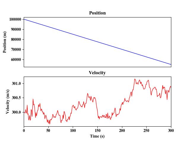
# 04 估计距离与估计速度
plt.figure(4)
plt.subplot(2, 1, 1)
plt.plot(t, xKFPlot[0, :], 'b', linewidth=1)
plt.title('Position', fontdict=fontTitle)
plt.ylabel('Position (m)', fontdict=font)
plt.tick_params(pad=3)
plt.yticks(fontproperties='Times New Roman', size=10)
plt.xticks([], fontproperties='Times New Roman', size=10)
plt.xlim(0, T)

plt.subplot(2, 1, 2)
plt.plot(t, xKFPlot[1, :], 'r', linewidth=1)
plt.title('Velocity', fontdict=fontTitle)
plt.xlabel('Time (s)', fontdict=font), plt.ylabel('Velocity (m/s)', fontdict=font)
plt.tick_params(pad=3)
plt.yticks(fontproperties='Times New Roman', size=10)
plt.xticks(fontproperties='Times New Roman', size=10)
plt.xlim(0, T)

plt.show()

仿真结果图如下所示。

用卡尔曼滤波器跟踪导弹（给出matlab和python的仿真代码） - 文章图片

? ? ? E n d ? ? ? ---End--- ???End???

内容总结

以上是互联网集市为您收集整理的用卡尔曼滤波器跟踪导弹（给出matlab和python的仿真代码）全部内容，希望文章能够帮你解决用卡尔曼滤波器跟踪导弹（给出matlab和python的仿真代码）所遇到的程序开发问题。如果觉得互联网集市技术教程内容还不错，欢迎将互联网集市网站推荐给程序员好友。

内容备注

版权声明：本文内容由互联网用户自发贡献，该文观点与技术仅代表作者本人。本站仅提供信息存储空间服务，不拥有所有权，不承担相关法律责任。如发现本站有涉嫌侵权/违法违规的内容，请发送邮件至 gblab@vip.qq.com 举报，一经查实，本站将立刻删除。

内容手机端

扫描二维码推送至手机访问。

本文链接：https://qyyshop.com/info/589372.html

来源：【匿名】

【上一篇】python自动化测试——Selenium Grid（二）【下一篇】浅谈PHP运行Python脚本的方法

更多 ►

【用卡尔曼滤波器跟踪导弹（给出matlab和python的仿真代码）】教程文章相关的互联网学习教程文章

python代码项目篇-银行三次登录锁定测试

cat account.txt ——用户密码名册jack pass1marry pass2natasha pass3touch lock.txt ——用户锁文件cat login.py#!/usr/bin/env pythonimport tab#put account.txt infomationf = file(‘account.txt‘)account_list = f.readlines()f.close()f = file(‘lock.txt‘)lock_list = []for i in f.readlines(): line = i.strip() lock_list.append(line)f.close()for i in range(3): userlogin ...

一些 Python 代码加速运行的技巧进行整理【图】

前言本文的文字及图片来源于网络,仅供学习、交流使用,不具有任何商业用途,版权归原作者所有,如有问题请及时联系我们以作处理。基本环境配置版本：Python3系统：Windows 需要安装：1.JDK - Download JDK，Appium要求用户必须配置JAVA环境, 否则启动Seesion报错。2.Appium - Download Appium, 安装过程请自行搜索。3.Android SDK - Download SDK4. Selenium - 建议使用低版本的Python Selenium库，在Chrome高版本可能会报错。例如： ...

Python爬取博客园新闻代码【代码】【图】

核心模块：requests ：安装指令 pip3 install requestsBeautifulSoup :安装指令 pip3 install beautifulsoup4代码：import requests import bs4 import osresponse=requests.get(‘https://news.cnblogs.com/‘) response.encoding=response.apparent_encodingfrom bs4 import BeautifulSoup soup=bs4.BeautifulSoup(response.text,features=‘html.parser‘) newslist=soup.find_all(‘div‘,class_="content") #print(newslist)f...

用Python写的图片蜘蛛人代码

复制代码代码如下:#coding=utf-8 import os import sys import re import urllib URL_REG = re.compile(r‘(http://[^///]+)‘, re.I) IMG_REG = re.compile(r‘<img[^>]*?src=([/‘"])([^/1]*?)/1‘, re.I) def download(dir, url): ‘‘‘下载网页中的图片 @dir 保存到本地的路径 @url 网页url ‘‘‘ global URL_REG, IMG_REG m = URL_REG.match(url) if not m: print ‘[Error]Invalid URL: ‘, url return host = m.group(1)...

在RPA中优雅地写Python代码（一）【代码】

人生苦短，我用Python！Python 是一种代表简单思想的语言，其语法相对简单，很容易上手。不过，如果就此小视 Python 语法的精妙和深邃，那就大错特错了。在RPA设计中，难免少不了一些简单的代码编写，本文精心筛选了最能展现 Python 语法之精妙的几个知识点，若是能够融会贯通、灵活使用，必将使代码更为精炼、高效，同时也会极大提升代码 B 格，使之看上去更老练，读起来更优雅。1. for - else什么？不是说if 和 else 才是原配吗...

Python外壳：代码结构

使用zip()并行迭代days = [‘Monday‘, ‘Tuesday‘, ‘Wednesday‘]>>> fruits = [‘banana‘, ‘orange‘, ‘peach‘]>>> drinks = [‘coffee‘, ‘tea‘, ‘beer‘]>>> desserts = [‘tiramisu‘, ‘ice cream‘, ‘pie‘, ‘pudding‘]>>> for day, fruit, drink, dessert in zip(days, fruits, drinks, desserts):... print(day, ": drink", drink, "- eat", fruit, "- enjoy", dessert)...Monday : drink coffee - eat banan...

字节转成k,M,G等python代码【代码】

def bytes2human(n):symbols = (‘K‘, ‘M‘, ‘G‘, ‘T‘, ‘P‘, ‘E‘, ‘Z‘, ‘Y‘)prefix = {}for i, s in enumerate(symbols):prefix[s] = 1 << (i + 1) * 10for s in reversed(symbols):if n >= prefix[s]:value = float(n) / prefix[s]return ‘%.1f%s‘ % (value,s)return ‘%sB‘ % n 原文：https://www.cnblogs.com/superniao/p/10554351.html

python代码编辑器PyCharm快捷键补充【图】

使用Pycharm的筒子们都知道查找快捷键是：Ctrl+F,你们知道替换吗？查了好久，都没有替换的快捷键，偶然发现了竟然是，Ctr+R 个人觉得特别有用的：替换：Ctrl+R 删除当前行 CTRY Y: 复制当前行：Ctrl+D ALT F7: 查找哪些地方使用了选中的方法。 ALT UP:移到上一个方法 ALT DOWN:移到下一个方法 CTRL SHIFT UP: 将当前行上移一行 CTRL SHIFT UP: 将当前行下移一行其他常用的一...

用Python自动清理电脑内重复文件，只要10行代码就够了【代码】

给定一个文件夹，使用Python检查给定文件夹下有无文件重复，若存在重复则删除主要涉及的知识点有：os模块综合应用glob模块综合应用利用filecmp模块比较两个文件步骤分析该程序实现的逻辑可以具化为：遍历获取给定文件夹下的所有文件，然后通过嵌套循环两两比较文件是否相同，如果相同则删除后者。实现问题的关键就变成了如何判断两个文件是否相同？在这里我们可以使用filecmp模块，来看看官方的介绍文档：filecmp.cmp(f1, f2, shal...

Python - 使用Pylint检查分析代码【代码】【图】

1-简介Home Page : https://www.pylint.org/检查语法错误，是否遵守编码风格标准、潜在的问题等；支持自定义配置：例如显示或隐藏特定的警告，并且可以通过编写插件来添加功能；使用Pylint检查文件时，需要直接将模块或包名作为参数；可以在命令行以脚本方式运行（pylint），也可作为模块（pylint.lint）导入，建议作为命令行工具使用； 2-帮助信息帮助信息：在命令行下运行“pylint -h”或“pylint --help”获取帮助信息；常用命令...

python代码进入谷歌浏览器手机模式【代码】

from selenium import webdrivermobileEmulation = {‘deviceName‘ :‘Galaxy S5‘}option = webdriver.ChromeOptions()option.add_experimental_option(‘mobileEmulation‘,mobileEmulation)charome = webdriver.Chrome(options=option）网上找到的都是这种方式，但这种方法有些弊端，这个没有真正进入toggle device toolbar模式，导致后续有些操作无法实现。目前还没找到方法去：模拟打开开发者模式，再点击oggle device tool...

Redis代码——Python篇【代码】

需要安装的库：redisimport redis# 连接数据库 r = redis.StrictRedis(host="localhost", port=6379, password="密码")# 方法1：根据数据类型的不同，调用响应的方法 # 写 r.set("p1", "good") # 读print(r.get("p1")) 原文：https://www.cnblogs.com/Rain2017/p/10335083.html

Python基本图形绘制练习题代码记录【代码】

样例Python蛇#PythonDraw.py #调用turtle库import turtle #设置窗口大小（窗口长度、窗口宽度、窗口距离屏幕的距离） turtle.setup(650,350,200,200) #penup抬起画笔turtle.penup() #fd向后画250个像素的直线 turtle.fd(-250) #pendown放下画笔turtle.pendown() #pensize画笔尺寸为25个像素 turtle.pensize(25) #pencolor画笔颜色函数 turtle.pencolor("purple") #seth函数全程为setheading(angle)：控制海龟角度 turtle.seth(-40)...

怎么让你的代码更Pythonic?光有技巧可不行，你还需要看这些

写代码如同写文章，好的文章是反复修改出来的，代码也同样是反复的重构出来的。今天给大家分享下，怎么从一个编程学习者变为一个程序猿（程序媛）！起码不要让别人一看你的代码就知道你是个小菜鸟！我们通常写一个代码，必然会经过一个简单-难-简洁的过程，那么在重构的过程中需要注意哪些呢？1、代码可以正常运行首先必然要保证，代码可以正常运行！不论你是直接按逻辑写下来还是函数式编程，必须先能实现你的代码功能，可以正常...

数论：任意数求原根（python代码）【代码】【图】

# 用辗转相除求最大公因子def gcd(a,b):r=a%bwhile(r!=0):a=bb=rr=a%breturn b# 欧拉函数-暴力循环版def euler(a):count=0for i in range(1,a):if gcd(a,i)==1:count+=1return countdef order(a,n,b): # 输出b在mod(a)中的阶 # n是mod(a)群的阶p=1while(p<=n and (b**p%a!=1)):p+=1if p<=n:return pelse:return -1# 求任意数原根def primitive_root(a):n=euler(a)prim=[]for b in range(2,a):if order(a,n,b)==n:prim.append(b...

PYTHON - 技术教程分类

Python3 教程 Python3 简介 Python3 环境搭建 Python3 基础语法 Python3 基本数据类型 Python3 解释器 Python3 注释 Python3 运算符 Python3 数字(Number) Python3 字符串 Python3 列表 Python3 元组 Python3 字典 Python3 集合 Python3 编程第一步 Python3 条件控制 Python3 循环语句 Python3 迭代器与生成器 Python3 函数 Python3 数据结构 Python3 模块 Python3 输入和输出 Python3 File Python3 OS Python3 错误和异常 Python3 面向对象 Python3 命名空间/作用域 Python3 标准库概览 Python3 实例 Python3 CGI编程 Python3 MySQL(PyMySQL) Python3 网络编程 Python3 SMTP发送邮件 Python3 多线程 Python3 日期和时间 Python3 内置函数 Python3 MongoDB Python3 urllib python 全部

PYTHON - 最热教程

python如何统计字符串中字母个数？使用Python进行微信公众号开发（三）回...Python+PyQT5的子线程更新UI界面的实例 python时间戳怎么获得？如何获得当前时...vscode调试python时提示无法将“conda”...python接口自动化全局变量access_token...python收取邮件(腾讯企业邮箱)python如何绘制降水图详解python并发获取snmp信息及性能测试...怎么卸载Python3.6？

首页 / PYTHON / 用卡尔曼滤波器跟踪导弹（给出matlab和python的仿真代码）

用卡尔曼滤波器跟踪导弹（给出matlab和python的仿真代码）

内容导读

内容图文

题目

matlab仿真代码

python仿真代码

内容总结

内容备注

内容手机端

【用卡尔曼滤波器跟踪导弹（给出matlab和python的仿真代码）】教程文章相关的互联网学习教程文章

python代码项目篇-银行三次登录锁定测试

一些 Python 代码加速运行的技巧进行整理【图】

Python爬取博客园新闻代码【代码】【图】

用Python写的图片蜘蛛人代码

在RPA中优雅地写Python代码（一）【代码】

Python外壳：代码结构

字节转成k,M,G等python代码【代码】

python代码编辑器PyCharm快捷键补充【图】

用Python自动清理电脑内重复文件，只要10行代码就够了【代码】

Python - 使用Pylint检查分析代码【代码】【图】

python代码进入谷歌浏览器手机模式【代码】

Redis代码——Python篇【代码】

Python基本图形绘制练习题代码记录【代码】

怎么让你的代码更Pythonic?光有技巧可不行，你还需要看这些

数论：任意数求原根（python代码）【代码】【图】

PYTHON - 相关标签

MATLAB - 相关标签

PYTHON - 技术教程分类

PYTHON - 最新教程

PYTHON - 最热教程