利用python实现梯度下降和逻辑回归原理(Python详细源码：预测学生是否被录取)

内容导读

互联网集市收集整理的这篇技术教程文章主要介绍了利用python实现梯度下降和逻辑回归原理(Python详细源码：预测学生是否被录取)，小编现在分享给大家，供广大互联网技能从业者学习和参考。文章包含5047字，纯文字阅读大概需要8分钟。

内容图文

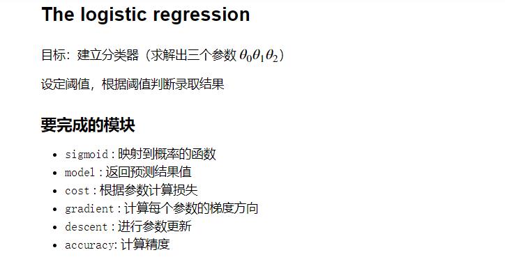
我们将建立一个逻辑回归模型来预测一个学生是否被大学录取。假设你是一个大学系的管理员，你想根据两次考试的结果来决定每个申请人的录取机会。你有以前的申请人的历史数据，你可以用它作为逻辑回归的训练集。对于每一个培训例子，你有两个考试的申请人的分数和录取决定。为了做到这一点，我们将建立一个分类模型，根据考试成绩估计入学概率。

导入函数库

#三大件
import numpy as np
import pandas as pd
import matplotlib.pyplot as plt
%matplotlib inline

导入数据，显示数据表头

import os
path = 'data' + os.sep + 'LogiReg_data.txt'
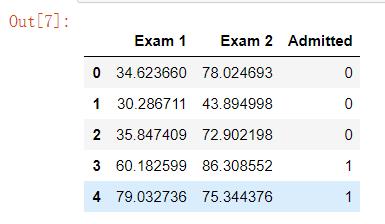
pdData = pd.read_csv(path, header=None, names=['Exam 1', 'Exam 2', 'Admitted'])
pdData.head()
pdData.shape
#看数据 的维度，100*3

结果：

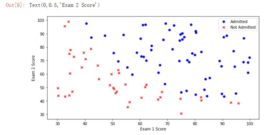
显示数据，画图

positive = pdData[pdData['Admitted'] == 1] # returns the subset of rows such Admitted = 1, i.e. the set of *positive* examples
negative = pdData[pdData['Admitted'] == 0] # returns the subset of rows such Admitted = 0, i.e. the set of *negative* examples

fig, ax = plt.subplots(figsize=(10,5)) #指定画图域
ax.scatter(positive['Exam 1'], positive['Exam 2'], s=30, c='b', marker='o', label='Admitted')
ax.scatter(negative['Exam 1'], negative['Exam 2'], s=30, c='r', marker='x', label='Not Admitted')
ax.legend()
ax.set_xlabel('Exam 1 Score')
ax.set_ylabel('Exam 2 Score')

结果：

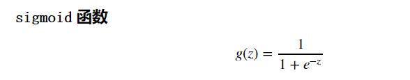
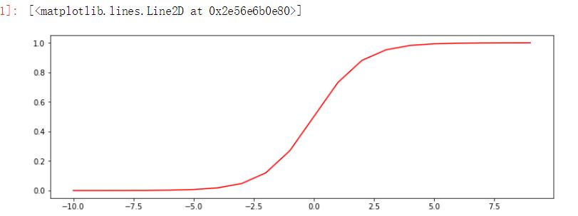
Sigmoid 函数

def sigmoid(z):
    return 1 / (1 + np.exp(-z))
    
nums = np.arange(-10, 10, step=1) #creates a vector containing 20 equally spaced values from -10 to 10
fig, ax = plt.subplots(figsize=(12,4))
ax.plot(nums, sigmoid(nums), 'r')

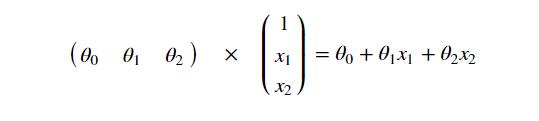
模型函数

def model(X, theta):
    """ Returns our model result
    :param X: examples to classify, n x p
    :param theta: parameters, 1 x p
    :return: the sigmoid evaluated for each examples in X given parameters theta as a n x 1 vector
    """
    return sigmoid(np.dot(X, theta.T))  # 矩阵乘法

pdData.insert(0, 'Ones', 1) # in a try / except structure so as not to return an error if the block si executed several times


# set X (training data) and y (target variable)
orig_data = pdData.as_matrix() # convert the Pandas representation of the data to an array useful for further computations
cols = orig_data.shape[1]
X = orig_data[:,0:cols-1] 
y = orig_data[:,cols-1:cols]

# convert to numpy arrays and initalize the parameter array theta
#X = np.matrix(X.values)
#y = np.matrix(data.iloc[:,3:4].values) #np.array(y.values)
theta = np.zeros([1, 3]) #占位 1*3，写一些检查一些

损失函数

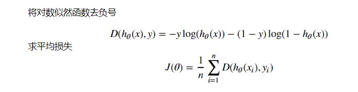
def cost(X, y, theta):  #数据，标签，估计
    left = np.multiply(-y, np.log(model(X, theta)))
    right = np.multiply(1 - y, np.log(1 - model(X, theta)))
    return np.sum(left - right) / (len(X))
cost(X, y, theta)

计算梯度

def gradient(X, y, theta):
    grad = np.zeros(theta.shape)
    error = (model(X, theta)- y).ravel()
    for j in range(len(theta.ravel())): #for each parmeter
        term = np.multiply(error, X[:,j])
        grad[0, j] = np.sum(term) / len(X)
    
    return grad

比较3中不同梯度下降方法

STOP_ITER = 0 #按照迭代次数进行停止
STOP_COST = 1 #按照目标函数的变化进行停止，无变化停止
STOP_GRAD = 2 #按照梯度变化，无变化停止

def stopCriterion(type, value, threshold):
    #设定三种不同的停止策略
    if type == STOP_ITER:        return value > threshold
    elif type == STOP_COST:      return abs(value[-1]-value[-2]) < threshold
    elif type == STOP_GRAD:      return np.linalg.norm(value) < threshold
import numpy.random

#洗牌 提高泛化能力
def shuffleData(data):
    np.random.shuffle(data) #随机模块，洗牌函数
    cols = data.shape[1]
    X = data[:, 0:cols-1] #数据
    y = data[:, cols-1:]  #标签
    return X, y

import time

def descent(data, theta, batchSize, stopType, thresh, alpha):
    #梯度下降求解
    
    init_time = time.time()
    i = 0 # 迭代次数
    k = 0 # batch
    X, y = shuffleData(data)
    grad = np.zeros(theta.shape) # 计算的梯度
    costs = [cost(X, y, theta)] # 损失值

    
    while True:
        grad = gradient(X[k:k+batchSize], y[k:k+batchSize], theta)
        k += batchSize #取batch数量个数据
        if k >= n: 
            k = 0 
            X, y = shuffleData(data) #重新洗牌
        theta = theta - alpha*grad # 参数更新
        costs.append(cost(X, y, theta)) # 计算新的损失
        i += 1 

        if stopType == STOP_ITER:       value = i
        elif stopType == STOP_COST:     value = costs
        elif stopType == STOP_GRAD:     value = grad
        if stopCriterion(stopType, value, thresh): break
    
    return theta, i-1, costs, grad, time.time() - init_time

def runExpe(data, theta, batchSize, stopType, thresh, alpha):
    #import pdb; pdb.set_trace();
    theta, iter, costs, grad, dur = descent(data, theta, batchSize, stopType, thresh, alpha)
    name = "Original" if (data[:,1]>2).sum() > 1 else "Scaled"
    name += " data - learning rate: {} - ".format(alpha)
    if batchSize==n: strDescType = "Gradient"
    elif batchSize==1:  strDescType = "Stochastic"
    else: strDescType = "Mini-batch ({})".format(batchSize)
    name += strDescType + " descent - Stop: "
    if stopType == STOP_ITER: strStop = "{} iterations".format(thresh)
    elif stopType == STOP_COST: strStop = "costs change < {}".format(thresh)
    else: strStop = "gradient norm < {}".format(thresh)
    name += strStop
    print ("***{}\nTheta: {} - Iter: {} - Last cost: {:03.2f} - Duration: {:03.2f}s".format(
        name, theta, iter, costs[-1], dur))
    fig, ax = plt.subplots(figsize=(12,4))
    ax.plot(np.arange(len(costs)), costs, 'r')
    ax.set_xlabel('Iterations')
    ax.set_ylabel('Cost')
    ax.set_title(name.upper() + ' - Error vs. Iteration')
    return theta

内容总结

以上是互联网集市为您收集整理的利用python实现梯度下降和逻辑回归原理(Python详细源码：预测学生是否被录取)全部内容，希望文章能够帮你解决利用python实现梯度下降和逻辑回归原理(Python详细源码：预测学生是否被录取)所遇到的程序开发问题。 如果觉得互联网集市技术教程内容还不错，欢迎将互联网集市网站推荐给程序员好友。

内容备注

版权声明：本文内容由互联网用户自发贡献，该文观点与技术仅代表作者本人。本站仅提供信息存储空间服务，不拥有所有权，不承担相关法律责任。如发现本站有涉嫌侵权/违法违规的内容， 请发送邮件至 gblab@vip.qq.com 举报，一经查实，本站将立刻删除。

内容手机端