首页 / 深度学习 / 深度学习之长短时记忆网络(LSTM)
深度学习之长短时记忆网络(LSTM)
内容导读
互联网集市收集整理的这篇技术教程文章主要介绍了深度学习之长短时记忆网络(LSTM),小编现在分享给大家,供广大互联网技能从业者学习和参考。文章包含34449字,纯文字阅读大概需要50分钟。
内容图文
")
本文转自《零基础入门深度学习》系列文章,阅读原文请移步这里
之前我们介绍了循环神经网络以及它的训练算法。我们也介绍了循环神经网络很难训练的原因,这导致了它在实际应用中,很难处理长距离的依赖。在本文中,我们将介绍一种改进之后的循环神经网络:长短时记忆网络(Long Short Term Memory Network, LSTM),它成功的解决了原始循环神经网络的缺陷,成为当前最流行的RNN,在语音识别、图片描述、自然语言处理等许多领域中成功应用。但不幸的一面是,LSTM的结构很复杂,因此,我们需要花上一些力气,才能把LSTM以及它的训练算法弄明白。在搞清楚LSTM之后,我们再介绍一种LSTM的变体:GRU (Gated Recurrent Unit)。 它的结构比LSTM简单,而效果却和LSTM一样好,因此,它正在逐渐流行起来。最后,我们仍然会动手实现一个LSTM。
一、长短时记忆网络是啥
我们首先了解一下长短时记忆网络产生的背景。回顾一下《深度学习之循环神经网络(RNN)》中推导的,误差项沿时间反向传播的公式: δ k T = δ t T ∏ i = k t ? 1 d i a g [ f ′ ( n e t i ) ] W \delta_k^T= \delta_t^T\prod_{i=k}^{t-1}diag[f'(net_i)]W δkT?=δtT?i=k∏t?1?diag[f′(neti?)]W我们可以根据下面的不等式,来获取 δ k T \delta_k^T δkT?的模的上界(模可以看做对 δ k T \delta_k^T δkT?中每一项值的大小的度量): ∥ δ k T ∥ ? ∥ δ t T ∥ ∏ i = k t ? 1 ∥ W ∥ ∥ d i a g [ f ′ ( n e t i ) ] ∥ \lVert\delta_k^T\rVert\leqslant\lVert\delta_t^T\rVert\prod_{i=k}^{t-1}\lVert W \rVert\lVert diag[f'(net_i)]\rVert ∥δkT?∥?∥δtT?∥i=k∏t?1?∥W∥∥diag[f′(neti?)]∥ ? ∥ δ t T ∥ ( β W β f ) t ? k \leqslant\lVert\delta_t^T\rVert(\beta_W\beta_f)^{t-k}\space\space\space\space\space\space\space\space\space\space\space\space\space ?∥δtT?∥(βW?βf?)t?k 我们可以看到,误差项 δ \delta δ从t时刻传递到k时刻,其值的上界是 β f β w \beta_f\beta_w βf?βw?的指数函数。 β f β w \beta_f\beta_w βf?βw?分别是对角矩阵 d i a g [ f ′ ( n e t i ) ] diag[f'(net_i)] diag[f′(neti?)]和矩阵 W W W模的上界。显然,除非 β f β w \beta_f\beta_w βf?βw?乘积的值位于1附近,否则,当t-k很大时(也就是误差传递很多个时刻时),整个式子的值就会变得极小(当 β f β w \beta_f\beta_w βf?βw?乘积小于1)或者极大(当 β f β w \beta_f\beta_w βf?βw?乘积大于1),前者就是梯度消失,后者就是梯度爆炸。虽然科学家们搞出了很多技巧(比如怎样初始化权重),让的值尽可能贴近于1,终究还是难以抵挡指数函数的威力。
梯度消失到底意味着什么?在《深度学习之循环神经网络(RNN)》中我们已证明,权重数组W最终的梯度是各个时刻的梯度之和,即:
?
W
E
=
∑
i
=
1
t
?
W
t
E
\nabla_{W}E=\sum_{i=1}^t\nabla_{W_t}E\space\space\space\space\space\space\space\space\space\space\space\space\space\space\space\space\space\space\space\space\space\space\space\space\space
?W?E=i=1∑t??Wt??E
=
?
W
t
E
+
?
W
t
?
1
E
+
.
.
.
+
?
W
1
E
\space\space\space\space\space\space\space\space\space\space\space\space\space\space\space\space\space\space\space\space\space\space=\nabla_{W_t}E+\nabla_{W_{t-1}}E+...+\nabla_{W_1}E
=?Wt??E+?Wt?1??E+...+?W1??E假设某轮训练中,各时刻的梯度以及最终的梯度之和如下图: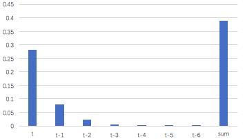
我们就可以看到,从上图的t-3时刻开始,梯度已经几乎减少到0了。那么,从这个时刻开始再往之前走,得到的梯度(几乎为零)就不会对最终的梯度值有任何贡献,这就相当于无论t-3时刻之前的网络状态h是什么,在训练中都不会对权重数组W的更新产生影响,也就是网络事实上已经忽略了t-3时刻之前的状态。这就是原始RNN无法处理长距离依赖的原因。
既然找到了问题的原因,那么我们就能解决它。从问题的定位到解决,科学家们大概花了7、8年时间。终于有一天,Hochreiter和Schmidhuber两位科学家发明出长短时记忆网络,一举解决这个问题。
其实,长短时记忆网络的思路比较简单。原始RNN的隐藏层只有一个状态,即h,它对于短期的输入非常敏感。那么,假如我们再增加一个状态,即c,让它来保存长期的状态,那么问题不就解决了么?如下图所示:
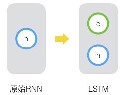
新增加的状态c,称为单元状态(cell state)。我们把上图按照时间维度展开:
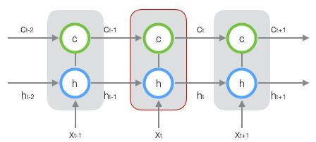
上图仅仅是一个示意图,我们可以看出,在t时刻,LSTM的输入有三个:当前时刻网络的输入值
x
t
\mathbf{x}_t
xt?、上一时刻LSTM的输出值
h
t
?
1
\mathbf{h}_{t-1}
ht?1?、以及上一时刻的单元状态
c
t
?
1
\mathbf{c}_{t-1}
ct?1?;LSTM的输出有两个:当前时刻LSTM输出值
h
t
\mathbf{h}_{t}
ht?、和当前时刻的单元状态
c
t
\mathbf{c}_{t}
ct?。注意
x
、
h
、
c
\mathbf{x}、\mathbf{h}、\mathbf{c}
x、h、c都是向量。
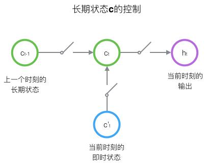
LSTM的关键,就是怎样控制长期状态
c
c
c。在这里,LSTM的思路是使用三个控制开关。第一个开关,负责控制继续保存长期状态
c
c
c;第二个开关,负责控制把即时状态输入到长期状态
c
c
c;第三个开关,负责控制是否把长期状态
c
c
c作为当前的LSTM的输出。三个开关的作用如下图所示:
接下来,我们要描述一下,输出h和单元状态c的具体计算方法。
二、长短时记忆网络的前向计算
前面描述的开关是怎样在算法中实现的呢?这就用到了门(gate)的概念。门实际上就是一层全连接层,它的输入是一个向量,输出是一个0到1之间的实数向量。假设 W W W是门的权重向量, b \mathbf{b} b是偏置项,那么门可以表示为: g ( x ) = σ ( W x + b ) g(x)=\sigma(W\mathbf{x}+\mathbf{b}) g(x)=σ(Wx+b)门的使用,就是用门的输出向量按元素乘以我们需要控制的那个向量。因为门的输出是0到1之间的实数向量,那么,当门输出为0时,任何向量与之相乘都会得到0向量,这就相当于啥都不能通过;输出为1时,任何向量与之相乘都不会有任何改变,这就相当于啥都可以通过。因为 σ \sigma σ(也就是sigmoid函数)的值域是(0,1),所以门的状态都是半开半闭的。
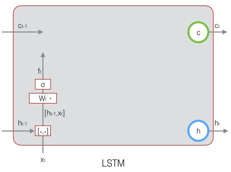
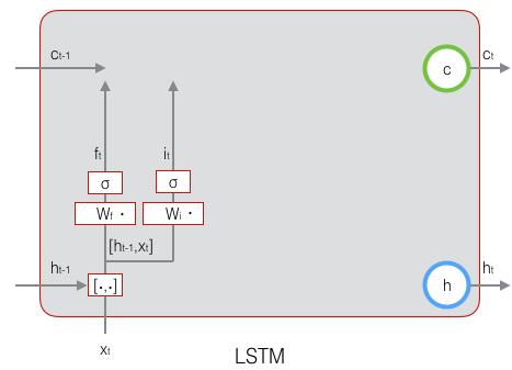
LSTM用两个门来控制单元状态 c c c的内容,一个是遗忘门(forget gate),它决定了上一时刻的单元状态 c t ? 1 \mathbf{c}_{t-1} ct?1?有多少保留到当前时刻 c t \mathbf{c}_{t} ct?;另一个是输入门(input gate),它决定了当前时刻网络的输入 x t \mathbf{x}_t xt?有多少保存到单元状态 c t \mathbf{c}_t ct?。LSTM用输出门(output gate)来控制单元状态 c t \mathbf{c}_t ct?有多少输出到LSTM的当前输出值 h t \mathbf{h}_t ht?。
我们先来看一下遗忘门:
f
t
=
σ
(
W
f
?
[
h
t
?
1
,
x
t
]
+
b
f
)
(
式
1
)
\mathbf{f}_t=\sigma(W_f·[\mathbf{h}_{t-1},\mathbf{x}_t]+\mathbf{b}_f)\space\space\space\space\space\space(式1)
ft?=σ(Wf??[ht?1?,xt?]+bf?) (式1)上式中,
W
f
W_f
Wf?是遗忘门的权重矩阵,
[
h
t
?
1
,
x
t
]
[\mathbf{h}_{t-1},\mathbf{x}_t]
[ht?1?,xt?]表示把两个向量连接成一个更长的向量,
b
f
\mathbf{b}_f
bf?是遗忘门的偏置项,
σ
\sigma
σ是sigmoid函数。如果输入的维度是
d
x
d_x
dx?,隐藏层的维度是
d
h
d_h
dh?,单元状态的维度是
d
c
d_c
dc?(通常
d
c
=
d
h
d_c=d_h
dc?=dh?),则遗忘门的权重矩阵
W
f
W_f
Wf?维度是
d
c
×
(
d
h
+
d
x
)
d_c\times (d_h+d_x)
dc?×(dh?+dx?)。事实上,权重矩阵
W
f
W_f
Wf?都是两个矩阵拼接而成的:一个是
W
f
h
W_{fh}
Wfh?,它对应着输入项
h
t
?
1
\mathbf{h}_{t-1}
ht?1?,其维度为
d
c
×
d
h
d_c\times d_h
dc?×dh?;一个是
W
f
x
W_{fx}
Wfx?,它对应着输入项
x
t
\mathbf{x}_t
xt?,其维度为
d
c
×
d
x
d_c \times d_x
dc?×dx?。
W
f
W_f
Wf?可以写为:
[
W
f
]
[
h
t
?
1
x
t
]
=
[
W
f
h
W
f
x
]
[
h
t
?
1
x
t
]
[W_f]\begin{bmatrix} \mathbf{h}_{t-1} \\ \mathbf{x}_t \end{bmatrix}=\begin{bmatrix} W_{fh}\space\space W_{fx}\end{bmatrix}\begin{bmatrix} \mathbf{h}_{t-1} \\ \mathbf{x}_t\end{bmatrix}\space\space\space\space\space\space\space\space\space\space\space\space
[Wf?][ht?1?xt??]=[Wfh? Wfx??][ht?1?xt??]
=
W
f
h
h
t
?
1
+
W
f
x
x
t
\space\space\space\space\space\space\space=W_{fh}\mathbf{h}_{t-1}+W_{fx}\mathbf{x}_t
=Wfh?ht?1?+Wfx?xt?下图显示了遗忘门的计算:
接下来看看输入门:
i
t
=
σ
(
W
i
?
[
h
t
?
1
,
x
t
]
+
b
i
)
(
式
2
)
\mathbf{i}_t=\sigma(W_i·[\mathbf{h}_{t-1},\mathbf{x}_t]+\mathbf{b}_i)\space\space\space\space\space\space(式2)
it?=σ(Wi??[ht?1?,xt?]+bi?) (式2)上式中,
W
i
W_i
Wi?是输入门的权重矩阵,
b
i
\mathbf{b}_i
bi?是输入门的偏置项。下图表示了输入门的计算:
接下来,我们计算用于描述当前输入的单元状态
c
~
t
\tilde \mathbf{c}_t
c~t?,它是根据上一次的输出和本次输入来计算的:
c
~
t
=
t
a
n
h
(
W
c
?
[
h
t
?
1
,
x
t
]
+
b
c
)
(
式
3
)
\tilde \mathbf{c}_t=tanh(W_c·[\mathbf{h}_{t-1},\mathbf{x}_t] + \mathbf{b}_c)\space\space\space\space\space\space(式3)
c~t?=tanh(Wc??[ht?1?,xt?]+bc?) (式3)下图是
c
~
t
\tilde \mathbf{c}_t
c~t?的计算:

现在,我们计算当前时刻的单元状态
c
t
\mathbf{c}_t
ct?。它是由上一次的单元状态
c
t
?
1
\mathbf{c}_{t-1}
ct?1?按元素乘以遗忘门
f
t
f_t
ft?,再用当前输入的单元状态
c
~
t
\tilde \mathbf{c}_t
c~t?按元素乘以输入门
i
t
i_t
it?,再将两个积加和产生的:
c
t
=
f
t
°
c
?
1
+
i
t
°
c
~
t
(
式
4
)
\mathbf{c}_t=f_t\circ \mathbf{c}_{-1}+i_t \circ \tilde \mathbf{c}_t\space\space\space\space\space\space(式4)
ct?=ft?°c?1?+it?°c~t? (式4)符号
°
\circ
°表示按元素乘。下图是
c
t
\mathbf{c}_t
ct?的计算: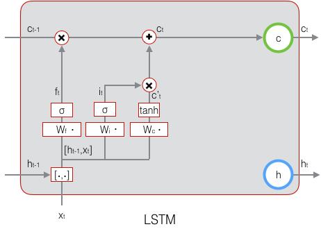
这样,我们就把LSTM关于当前的记忆
c
~
t
\tilde \mathbf{c}_t
c~t?和长期的记忆
c
t
?
1
\mathbf{c}_{t-1}
ct?1?组合在一起,形成了新的单元状态
c
t
\mathbf{c}_t
ct?。由于遗忘门的控制,它可以保存很久很久之前的信息,由于输入门的控制,它又可以避免当前无关紧要的内容进入记忆。下面,我们要看看输出门,它控制了长期记忆对当前输出的影响:
o
t
=
σ
(
W
o
?
[
h
t
?
1
,
x
t
]
+
b
o
)
(
式
5
)
\mathbf{o}_t=\sigma(W_o·[\mathbf{h}_{t-1}, \mathbf{x}_t]+\mathbf{b}_o)\space\space\space\space\space\space(式5)
ot?=σ(Wo??[ht?1?,xt?]+bo?) (式5)下图表示输出门的计算: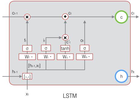
LSTM最终的输出,是由输出门和单元状态共同确定的:
h
t
=
o
t
°
t
a
n
h
(
c
t
)
(
式
6
)
\mathbf{h}_t=\mathbf{o}_t \circ tanh(\mathbf{c}_t)\space\space\space\space\space\space(式6)
ht?=ot?°tanh(ct?) (式6)下图表示LSTM最终输出的计算:
(式1)到(式6)就是LSTM前向计算的全部公式。至此,我们就把LSTM前向计算讲完了。
三、长短时记忆网络的训练
熟悉我们这个系列文章的同学都清楚,训练部分往往比前向计算部分复杂多了。LSTM的前向计算都这么复杂,那么,可想而知,它的训练算法一定是非常非常复杂的。现在只有做几次深呼吸,再一头扎进公式海洋吧。
LSTM训练算法框架
LSTM的训练算法仍然是反向传播算法,对于这个算法,我们已经非常熟悉了。主要有下面三个步骤:
- 前向计算每个神经元的输出值,对于LSTM来说,即 f t 、 i t 、 c t 、 o t 、 h t \mathbf{f}_t、\mathbf{i}_t、\mathbf{c}_t、\mathbf{o}_t、\mathbf{h}_t ft?、it?、ct?、ot?、ht?五个向量的值。计算方法已经在上一节中描述过了。
- 反向计算每个神经元的误差项 δ \delta δ值。与循环神经网络一样,LSTM误差项的反向传播也是包括两个方向:一个是沿时间的反向传播,即从当前t时刻开始,计算每个时刻的误差项;一个是将误差项向上一层传播。
- 根据相应的误差项,计算每个权重的梯度。
关于公式和符号的说明
首先,我们对推导中用到的一些公式、符号做一下必要的说明。
接下来的推导中,我们设定gate的激活函数为sigmoid函数,输出的激活函数为tanh函数。他们的导数分别为:
σ
(
z
)
=
y
=
1
1
+
e
?
z
\sigma(z)=y=\frac{1}{1+e^{-z}}
σ(z)=y=1+e?z1?
σ
′
(
z
)
=
y
(
1
?
y
)
\sigma'(z)=y(1-y)\space\space\space\space\space\space\space\space
σ′(z)=y(1?y)
t
a
n
h
(
z
)
=
y
=
e
z
?
e
?
z
e
z
+
e
?
z
tanh(z)=y=\frac{e^z-e^{-z}}{e^z+e^{-z}}\space\space\space\space
tanh(z)=y=ez+e?zez?e?z?
t
a
n
h
′
(
z
)
=
1
?
y
2
tanh'(z)=1-y^2\space\space\space\space\space\space\space\space\space\space\space\space\space\space\space\space\space
tanh′(z)=1?y2 从上面可以看出,sigmoid和tanh函数的导数都是原函数的函数。这样,我们一旦计算原函数的值,就可以用它来计算出导数的值。
LSTM需要学习的参数共有8组,分别是:遗忘门的权重矩阵 W f W_f Wf?和偏置项 b f \mathbf{b}_f bf?、输入门的权重矩阵 W i W_i Wi?和偏置项 b i \mathbf{b}_i bi?、输出门的权重矩阵 W o W_o Wo?和偏置项 b o \mathbf{b}_o bo?,以及计算单元状态的权重矩阵 W c W_c Wc?和偏置项 b c \mathbf{b}_c bc?。因为权重矩阵的两部分在反向传播中使用不同的公式,因此在后续的推导中,权重矩阵 W f 、 W i 、 W o 、 W c W_f、W_i、W_o、W_c Wf?、Wi?、Wo?、Wc?都将被写为分开的两个矩阵: W f h 、 W f x 、 W i h 、 W i x 、 W o h 、 W o x 、 W c h 、 W c x W_{fh}、W_{fx}、W_{ih}、W_{ix}、W_{oh}、W_{ox}、W_{ch}、W_{cx} Wfh?、Wfx?、Wih?、Wix?、Woh?、Wox?、Wch?、Wcx?。
我们解释一下按元素乘 ° \circ °符号。当 ° \circ °作用于两个向量时,运算如下: a ° b = [ a 1 a 2 a 3 . . . a n ] ° [ b 1 b 2 b 3 . . . b n ] = [ a 1 b 1 a 2 b 2 a 3 b 3 . . . a n b n ] a \circ b=\begin{bmatrix} a_1 \\ a_2\\ a_3\\...\\a_n \end{bmatrix} \circ \begin{bmatrix} b_1 \\ b_2\\ b_3\\...\\b_n \end{bmatrix} = \begin{bmatrix} a_1b_1 \\ a_2b_2\\ a_3b_3\\...\\a_nb_n \end{bmatrix} a°b=???????a1?a2?a3?...an?????????°???????b1?b2?b3?...bn?????????=???????a1?b1?a2?b2?a3?b3?...an?bn?????????当 ° \circ °作用于一个向量和一个矩阵时,运算如下: a ° X = [ a 1 a 2 a 3 . . . a n ] ° [ x 11 x 12 . . . x 1 n x 21 x 22 . . . x 2 n x 31 x 32 . . . x 3 n . . . x n 1 x n 2 . . . x n n ] a \circ X = \begin{bmatrix} a_1 \\ a_2\\ a_3\\...\\a_n \end{bmatrix} \circ \begin{bmatrix} x_{11} \space\space x_{12} \space...\space x_{1n}\\ x_{21}\space\space x_{22} \space...\space x_{2n}\\ x_{31}\space\space x_{32} \space...\space x_{3n}\\...\\x_{n1}\space\space x_{n2} \space...\space x_{nn} \end{bmatrix} a°X=???????a1?a2?a3?...an?????????°???????x11? x12? ... x1n?x21? x22? ... x2n?x31? x32? ... x3n?...xn1? xn2? ... xnn????????? = [ a 1 x 11 a 1 x 12 . . . a 1 x 1 n a 2 x 21 a 2 x 22 . . . a 2 x 2 n a 3 x 31 a 3 x 32 . . . a 3 x 3 n . . . a n x n 1 a n x n 2 . . . a n x n n ] \space\space\space\space\space\space\space\space\space\space=\begin{bmatrix} a_1x_{11} \space\space a_1x_{12} \space...\space a_1x_{1n}\\ a_2x_{21}\space\space a_2x_{22} \space...\space a_2x_{2n}\\ a_3x_{31}\space\space a_3x_{32} \space...\space a_3x_{3n}\\...\\a_nx_{n1}\space\space a_nx_{n2} \space...\space a_nx_{nn} \end{bmatrix} =???????a1?x11? a1?x12? ... a1?x1n?a2?x21? a2?x22? ... a2?x2n?a3?x31? a3?x32? ... a3?x3n?...an?xn1? an?xn2? ... an?xnn?????????当 ° \circ °作用于两个矩阵时,两个矩阵对应位置的元素相乘。按元素乘可以在某些情况下简化矩阵和向量运算。例如,当一个对角矩阵右乘一个矩阵时,相当于用对角矩阵的对角线组成的向量按元素乘那个矩阵: d i a g [ a ] X = a ° X diag[a]X=a \circ X diag[a]X=a°X当一个行向量右乘一个对角矩阵时,相当于这个行向量按元素乘那个矩阵对角线组成的向量: a T d i a g [ b ] = a ° b a^Tdiag[b]=a \circ b aTdiag[b]=a°b上面这两点,在我们后续推导中会多次用到。
在t时刻,LSTM的输出值为 h t \mathbf{h}_t ht?。我们定义t时刻的误差项 δ t \delta_t δt?为: δ t = d e f ? E ? h t \delta_t\overset{def}{=}\frac{\partial E}{\partial \mathbf{h}_t} δt?=def?ht??E?注意,和前面几篇文章不同,我们这里假设误差项是损失函数对输出值的导数,而不是对加权输入 n e t t l net_t^l nettl?的导数。因为LSTM有四个加权输入,分别对应 f t 、 i t 、 c t 、 o t \mathbf{f}_t、\mathbf{i}_t、\mathbf{c}_t、\mathbf{o}_t ft?、it?、ct?、ot?,我们希望往上一层传递一个误差项而不是四个。但我们仍然需要定义出这四个加权输入,以及他们对应的误差项。 n e t f , t = W f [ h t ? 1 , x t ] + b f net_{f,t}=W_f[\mathbf{h}_{t-1},\mathbf{x}_t]+\mathbf{b}_f netf,t?=Wf?[ht?1?,xt?]+bf? = W f h h t ? 1 + W f x x t + b f \space\space\space\space\space\space\space\space\space\space\space\space\space\space\space\space\space\space\space\space=W_{fh}\mathbf{h}_{t-1}+W_{fx}\mathbf{x}_t+\mathbf{b}_f =Wfh?ht?1?+Wfx?xt?+bf? n e t i , t = W i [ h t ? 1 , x t ] + b i net_{i,t}=W_i[\mathbf{h}_{t-1},\mathbf{x}_t]+\mathbf{b}_i neti,t?=Wi?[ht?1?,xt?]+bi? = W i h h t ? 1 + W i x x t + b i \space\space\space\space\space\space\space\space\space\space\space\space\space\space\space\space\space\space\space=W_{ih}\mathbf{h}_{t-1}+W_{ix}\mathbf{x}_t+\mathbf{b}_i =Wih?ht?1?+Wix?xt?+bi? n e t c ~ , t = W c [ h t ? 1 , x t ] + b c net_{\tilde c,t}=W_c[\mathbf{h}_{t-1},\mathbf{x}_t]+\mathbf{b}_c netc~,t?=Wc?[ht?1?,xt?]+bc? = W c h h t ? 1 + W c x x t + b c \space\space\space\space\space\space\space\space\space\space\space\space\space\space\space\space\space\space\space=W_{ch}\mathbf{h}_{t-1}+W_{cx}\mathbf{x}_t+\mathbf{b}_c =Wch?ht?1?+Wcx?xt?+bc? n e t o , t = W o [ h t ? 1 , x t ] + b o net_{o,t}=W_o[\mathbf{h}_{t-1},\mathbf{x}_t]+\mathbf{b}_o neto,t?=Wo?[ht?1?,xt?]+bo? = W o h h t ? 1 + W o x x t + b o \space\space\space\space\space\space\space\space\space\space\space\space\space\space\space\space\space\space\space=W_{oh}\mathbf{h}_{t-1}+W_{ox}\mathbf{x}_t+\mathbf{b}_o =Woh?ht?1?+Wox?xt?+bo? δ f , t = d e f ? E ? n e t f , t \delta_{f,t}\overset{def}{=}\frac{\partial E}{\partial net_{f,t}} δf,t?=def?netf,t??E? δ i , t = d e f ? E ? n e t i , t \delta_{i,t}\overset{def}{=}\frac{\partial E}{\partial net_{i,t}} δi,t?=def?neti,t??E? δ c ~ , t = d e f ? E ? n e t c ~ , t \delta_{\tilde c,t}\overset{def}{=}\frac{\partial E}{\partial net_{\tilde c,t}} δc~,t?=def?netc~,t??E? δ o , t = d e f ? E ? n e t o , t \delta_{o,t}\overset{def}{=}\frac{\partial E}{\partial net_{o,t}} δo,t?=def?neto,t??E?
误差项沿时间的反向传递
沿时间反向传递误差项,就是要计算出t-1时刻的误差项
δ
t
?
1
\delta_{t-1}
δt?1?。
δ
t
?
1
T
=
?
E
?
h
t
?
1
\delta_{t-1}^T=\frac{\partial E}{\partial \mathbf{h}_{t-1}}
δt?1T?=?ht?1??E?
=
?
E
?
h
t
?
h
t
?
h
t
?
1
\space\space\space\space\space\space\space\space\space\space\space\space\space\space\space=\frac{\partial E}{\partial \mathbf{h}_{t}}\frac{\partial \mathbf{h}_t}{\partial \mathbf{h}_{t-1}}
=?ht??E??ht?1??ht??
=
δ
t
T
?
h
t
?
h
t
?
1
\space\space\space\space\space\space\space\space\space\space\space\space=\delta_t^T\frac{\partial \mathbf{h}_t}{\partial \mathbf{h}_{t-1}}
=δtT??ht?1??ht??我们知道,
?
h
t
?
h
t
?
1
\frac{\partial \mathbf{h}_t}{\partial \mathbf{h}_{t-1}}
?ht?1??ht??是一个Jacobian矩阵。如果隐藏层h的维度是N的话,那么它就是一个
N
×
N
N\times N
N×N矩阵。为了求出它,我们列出
h
t
\mathbf{h}_t
ht?的计算公式,即前面的(式6)和(式4):
h
t
=
o
t
°
t
a
n
h
(
c
t
)
\mathbf{h}_t=\mathbf{o}_t \circ tanh(\mathbf c_t)
ht?=ot?°tanh(ct?)
c
t
=
f
t
°
c
t
?
1
+
i
t
°
c
~
t
\space\space\space\space\space\space\space\space\space\mathbf c_t=\mathbf{f}_t \circ \space \mathbf c_{t-1}+\mathbf{i}_t\circ \space \tilde \mathbf{c}_t
ct?=ft?° ct?1?+it?° c~t?显然,
o
t
、
f
t
、
i
t
、
c
~
t
\mathbf{o}_t、\mathbf{f}_t、\mathbf{i}_t、\mathbf{\tilde{c}}_t
ot?、ft?、it?、c~t?都是
h
t
?
1
\mathbf{h}_{t-1}
ht?1?的函数,那么,利用全导数公式可得:
δ
t
T
?
h
t
?
h
t
?
1
=
δ
t
T
?
h
t
?
o
t
?
o
t
?
n
e
t
o
,
t
?
n
e
t
o
,
t
?
h
t
?
1
+
δ
t
T
?
h
t
?
c
t
?
c
t
?
f
t
?
f
t
?
n
e
t
f
,
t
?
n
e
t
f
,
t
?
h
t
?
1
+
δ
t
T
?
h
t
?
c
t
?
c
t
?
i
t
?
i
t
?
n
e
t
i
,
t
?
n
e
t
i
,
t
?
h
t
?
1
+
δ
t
T
?
h
t
?
c
t
?
c
t
?
c
~
t
?
c
~
t
?
n
e
t
c
~
,
t
?
n
e
t
c
~
,
t
?
h
t
?
1
\delta_t^T\frac{\partial{\mathbf{h_t}}}{\partial{\mathbf{h_{t-1}}}}=\delta_t^T\frac{\partial{\mathbf{h_t}}}{\partial{\mathbf{o}_t}}\frac{\partial{\mathbf{o}_t}}{\partial{\mathbf{net}_{o,t}}}\frac{\partial{\mathbf{net}_{o,t}}}{\partial{\mathbf{h_{t-1}}}} +\delta_t^T\frac{\partial{\mathbf{h_t}}}{\partial{\mathbf{c}_t}}\frac{\partial{\mathbf{c}_t}}{\partial{\mathbf{f_{t}}}}\frac{\partial{\mathbf{f}_t}}{\partial{\mathbf{net}_{f,t}}}\frac{\partial{\mathbf{net}_{f,t}}}{\partial{\mathbf{h_{t-1}}}} +\delta_t^T\frac{\partial{\mathbf{h_t}}}{\partial{\mathbf{c}_t}}\frac{\partial{\mathbf{c}_t}}{\partial{\mathbf{i_{t}}}}\frac{\partial{\mathbf{i}_t}}{\partial{\mathbf{net}_{i,t}}}\frac{\partial{\mathbf{net}_{i,t}}}{\partial{\mathbf{h_{t-1}}}} +\delta_t^T\frac{\partial{\mathbf{h_t}}}{\partial{\mathbf{c}_t}}\frac{\partial{\mathbf{c}_t}}{\partial{\mathbf{\tilde{c}}_{t}}}\frac{\partial{\mathbf{\tilde{c}}_t}}{\partial{\mathbf{net}_{\tilde{c},t}}}\frac{\partial{\mathbf{net}_{\tilde{c},t}}}{\partial{\mathbf{h_{t-1}}}}
δtT??ht?1??ht??=δtT??ot??ht???neto,t??ot???ht?1??neto,t??+δtT??ct??ht???ft??ct???netf,t??ft???ht?1??netf,t??+δtT??ct??ht???it??ct???neti,t??it???ht?1??neti,t??+δtT??ct??ht???c~t??ct???netc~,t??c~t???ht?1??netc~,t??
=
δ
o
,
t
T
?
n
e
t
o
,
t
?
h
t
?
1
+
δ
f
,
t
T
?
n
e
t
f
,
t
?
h
t
?
1
+
δ
i
,
t
T
?
n
e
t
i
,
t
?
h
t
?
1
+
δ
c
~
,
t
T
?
n
e
t
c
~
,
t
?
h
t
?
1
(
式
7
)
=\delta_{o,t}^T\frac{\partial{\mathbf{net}_{o,t}}}{\partial{\mathbf{h_{t-1}}}} +\delta_{f,t}^T\frac{\partial{\mathbf{net}_{f,t}}}{\partial{\mathbf{h_{t-1}}}} +\delta_{i,t}^T\frac{\partial{\mathbf{net}_{i,t}}}{\partial{\mathbf{h_{t-1}}}} +\delta_{\tilde{c},t}^T\frac{\partial{\mathbf{net}_{\tilde{c},t}}}{\partial{\mathbf{h_{t-1}}}}\qquad\quad(式7)
=δo,tT??ht?1??neto,t??+δf,tT??ht?1??netf,t??+δi,tT??ht?1??neti,t??+δc~,tT??ht?1??netc~,t??(式7)下面,我们要把(式7)中的每个偏导数都求出来。根据(式6),我们可以求出:
?
h
t
?
o
t
=
d
i
a
g
[
tanh
?
(
c
t
)
]
\frac{\partial{\mathbf{h_t}}}{\partial{\mathbf{o}_t}}=diag[\tanh(\mathbf{c}_t)]
?ot??ht??=diag[tanh(ct?)]
?
h
t
?
c
t
=
d
i
a
g
[
o
t
°
(
1
?
tanh
?
(
c
t
)
2
)
]
\space\space\space\space\space\space\space\space\space\space\space\space\space\space\space\space\space\space\space \frac{\partial{\mathbf{h_t}}}{\partial{\mathbf{c}_t}}=diag[\mathbf{o}_t\circ(1-\tanh(\mathbf{c}_t)^2)]
?ct??ht??=diag[ot?°(1?tanh(ct?)2)]根据(式4),我们可以求出:
?
c
t
?
f
t
=
d
i
a
g
[
c
t
?
1
]
\frac{\partial{\mathbf{c}_t}}{\partial{\mathbf{f_{t}}}}=diag[\mathbf{c}_{t-1}]
?ft??ct??=diag[ct?1?]
?
c
t
?
i
t
=
d
i
a
g
[
c
~
t
]
\frac{\partial{\mathbf{c}_t}}{\partial{\mathbf{i_{t}}}}=diag[\mathbf{\tilde{c}}_t]\space\space\space
?it??ct??=diag[c~t?]
?
c
t
?
c
~
t
=
d
i
a
g
[
i
t
]
\frac{\partial{\mathbf{c}_t}}{\partial{\mathbf{\tilde{c}_{t}}}}=diag[\mathbf{i}_t]\space\space\space\space
?c~t??ct??=diag[it?] 因为:
o
t
=
σ
(
n
e
t
o
,
t
)
\mathbf{o}_t=\sigma(\mathbf{net}_{o,t})\space\space\space\space\space\space\space\space\space\space\space\space\space\space\space\space\space\space
ot?=σ(neto,t?)
n
e
t
o
,
t
=
W
o
h
h
t
?
1
+
W
o
x
x
t
+
b
o
\mathbf{net}_{o,t}=W_{oh}\mathbf{h}_{t-1}+W_{ox}\mathbf{x}_t+\mathbf{b}_o
neto,t?=Woh?ht?1?+Wox?xt?+bo?
f
t
=
σ
(
n
e
t
f
,
t
)
\mathbf{f}_t=\sigma(\mathbf{net}_{f,t})\space\space\space\space\space\space\space\space\space\space\space\space\space\space\space\space\space
ft?=σ(netf,t?)
n
e
t
f
,
t
=
W
f
h
h
t
?
1
+
W
f
x
x
t
+
b
f
\mathbf{net}_{f,t}=W_{fh}\mathbf{h}_{t-1}+W_{fx}\mathbf{x}_t+\mathbf{b}_f
netf,t?=Wfh?ht?1?+Wfx?xt?+bf?
i
t
=
σ
(
n
e
t
i
,
t
)
\mathbf{i}_t=\sigma(\mathbf{net}_{i,t})\space\space\space\space\space\space\space\space\space\space\space\space\space\space\space\space\space
it?=σ(neti,t?)
n
e
t
i
,
t
=
W
i
h
h
t
?
1
+
W
i
x
x
t
+
b
i
\mathbf{net}_{i,t}=W_{ih}\mathbf{h}_{t-1}+W_{ix}\mathbf{x}_t+\mathbf{b}_i
neti,t?=Wih?ht?1?+Wix?xt?+bi?
c
~
t
=
tanh
?
(
n
e
t
c
~
,
t
)
\mathbf{\tilde{c}}_t=\tanh(\mathbf{net}_{\tilde{c},t})\space\space\space\space\space\space\space\space\space\space\space
c~t?=tanh(netc~,t?)
n
e
t
c
~
,
t
=
W
c
h
h
t
?
1
+
W
c
x
x
t
+
b
c
\mathbf{net}_{\tilde{c},t}=W_{ch}\mathbf{h}_{t-1}+W_{cx}\mathbf{x}_t+\mathbf{b}_c
netc~,t?=Wch?ht?1?+Wcx?xt?+bc?我们很容易得出:
?
o
t
?
n
e
t
o
,
t
=
d
i
a
g
[
o
t
°
(
1
?
o
t
)
]
\frac{\partial{\mathbf{o}_t}}{\partial{\mathbf{net}_{o,t}}}=diag[\mathbf{o}_t\circ(1-\mathbf{o}_t)]
?neto,t??ot??=diag[ot?°(1?ot?)]
?
n
e
t
o
,
t
?
h
t
?
1
=
W
o
h
\frac{\partial{\mathbf{net}_{o,t}}}{\partial{\mathbf{h_{t-1}}}}=W_{oh}\space\space\space\space\space\space\space\space\space\space\space\space\space\space\space\space\space\space\space\space\space\space\space
?ht?1??neto,t??=Woh?
?
f
t
?
n
e
t
f
,
t
=
d
i
a
g
[
f
t
°
(
1
?
f
t
)
]
\frac{\partial{\mathbf{f}_t}}{\partial{\mathbf{net}_{f,t}}}=diag[\mathbf{f}_t\circ(1-\mathbf{f}_t)]
?netf,t??ft??=diag[ft?°(1?ft?)]
?
n
e
t
f
,
t
?
h
t
?
1
=
W
f
h
\frac{\partial{\mathbf{net}_{f,t}}}{\partial{\mathbf{h}_{t-1}}}=W_{fh}\space\space\space\space\space\space\space\space\space\space\space\space\space\space\space\space\space\space\space\space\space\space
?ht?1??netf,t??=Wfh?
?
i
t
?
n
e
t
i
,
t
=
d
i
a
g
[
i
t
°
(
1
?
i
t
)
]
\frac{\partial{\mathbf{i}_t}}{\partial{\mathbf{net}_{i,t}}}=diag[\mathbf{i}_t\circ(1-\mathbf{i}_t)]
?neti,t??it??=diag[it?°(1?it?)]
?
n
e
t
i
,
t
?
h
t
?
1
=
W
i
h
\frac{\partial{\mathbf{net}_{i,t}}}{\partial{\mathbf{h}_{t-1}}}=W_{ih}\space\space\space\space\space\space\space\space\space\space\space\space\space\space\space\space\space\space\space\space\space
?ht?1??neti,t??=Wih?
?
c
~
t
?
n
e
t
c
~
,
t
=
d
i
a
g
[
1
?
c
~
t
2
]
\frac{\partial{\mathbf{\tilde{c}}_t}}{\partial{\mathbf{net}_{\tilde{c},t}}}=diag[1-\mathbf{\tilde{c}}_t^2]\space\space\space\space\space\space\space\space
?netc~,t??c~t??=diag[1?c~t2?]
?
n
e
t
c
~
,
t
?
h
t
?
1
=
W
c
h
\frac{\partial{\mathbf{net}_{\tilde{c},t}}}{\partial{\mathbf{h}_{t-1}}}=W_{ch}\space\space\space\space\space\space\space\space\space\space\space\space\space\space\space\space\space\space\space
?ht?1??netc~,t??=Wch? 将上述偏导数带入到(式7),我们得到:
δ
t
?
1
=
δ
o
,
t
T
?
n
e
t
o
,
t
?
h
t
?
1
+
δ
f
,
t
T
?
n
e
t
f
,
t
?
h
t
?
1
+
δ
i
,
t
T
?
n
e
t
i
,
t
?
h
t
?
1
+
δ
c
~
,
t
T
?
n
e
t
c
~
,
t
?
h
t
?
1
\delta_{t-1}=\delta_{o,t}^T\frac{\partial{\mathbf{net}_{o,t}}}{\partial{\mathbf{h_{t-1}}}} +\delta_{f,t}^T\frac{\partial{\mathbf{net}_{f,t}}}{\partial{\mathbf{h_{t-1}}}} +\delta_{i,t}^T\frac{\partial{\mathbf{net}_{i,t}}}{\partial{\mathbf{h_{t-1}}}} +\delta_{\tilde{c},t}^T\frac{\partial{\mathbf{net}_{\tilde{c},t}}}{\partial{\mathbf{h_{t-1}}}}
δt?1?=δo,tT??ht?1??neto,t??+δf,tT??ht?1??netf,t??+δi,tT??ht?1??neti,t??+δc~,tT??ht?1??netc~,t??
=
δ
o
,
t
T
W
o
h
+
δ
f
,
t
T
W
f
h
+
δ
i
,
t
T
W
i
h
+
δ
c
~
,
t
T
W
c
h
(
式
8
)
\space\space\space\space\space=\delta_{o,t}^T W_{oh} +\delta_{f,t}^TW_{fh} +\delta_{i,t}^TW_{ih} +\delta_{\tilde{c},t}^TW_{ch}\qquad\quad(式8)
=δo,tT?Woh?+δf,tT?Wfh?+δi,tT?Wih?+δc~,tT?Wch?(式8)根据
δ
o
,
t
、
δ
f
,
t
、
δ
i
,
t
、
δ
c
~
,
t
\delta_{o,t}、\delta_{f,t}、\delta_{i,t}、\delta_{\tilde{c},t}
δo,t?、δf,t?、δi,t?、δc~,t?的定义,可知:
δ
o
,
t
T
=
δ
t
T
°
tanh
?
(
c
t
)
°
o
t
°
(
1
?
o
t
)
(
式
9
)
\delta_{o,t}^T=\delta_t^T\circ\tanh(\mathbf{c}_t)\circ\mathbf{o}_t\circ(1-\mathbf{o}_t)\qquad\quad(式9)\space\space\space\space\space\space\space\space\space\space\space\space\space\space\space\space\space\space\space\space\space\space\space
δo,tT?=δtT?°tanh(ct?)°ot?°(1?ot?)(式9)
δ
f
,
t
T
=
δ
t
T
°
o
t
°
(
1
?
tanh
?
(
c
t
)
2
)
°
c
t
?
1
°
f
t
°
(
1
?
f
t
)
(
式
10
)
\space\space\space \delta_{f,t}^T=\delta_t^T\circ\mathbf{o}_t\circ(1-\tanh(\mathbf{c}_t)^2)\circ\mathbf{c}_{t-1}\circ\mathbf{f}_t\circ(1-\mathbf{f}_t)\qquad(式10)
δf,tT?=δtT?°ot?°(1?tanh(ct?)2)°ct?1?°ft?°(1?ft?)(式10)
δ
i
,
t
T
=
δ
t
T
°
o
t
°
(
1
?
tanh
?
(
c
t
)
2
)
°
c
~
t
°
i
t
°
(
1
?
i
t
)
(
式
11
)
\space\space\space \delta_{i,t}^T=\delta_t^T\circ\mathbf{o}_t\circ(1-\tanh(\mathbf{c}_t)^2)\circ\mathbf{\tilde{c}}_t\circ\mathbf{i}_t\circ(1-\mathbf{i}_t)\qquad\quad(式11)
δi,tT?=δtT?°ot?°(1?tanh(ct?)2)°c~t?°it?°(1?it?)(式11)
δ
c
~
,
t
T
=
δ
t
T
°
o
t
°
(
1
?
tanh
?
(
c
t
)
2
)
°
i
t
°
(
1
?
c
~
2
)
(
式
12
)
\delta_{\tilde{c},t}^T=\delta_t^T\circ\mathbf{o}_t\circ(1-\tanh(\mathbf{c}_t)^2)\circ\mathbf{i}_t\circ(1-\mathbf{\tilde{c}}^2)\qquad\quad(式12)\space\space\space\space
δc~,tT?=δtT?°ot?°(1?tanh(ct?)2)°it?°(1?c~2)(式12) (式8)到(式12)就是将误差沿时间反向传播一个时刻的公式。有了它,我们可以写出将误差项向前传递到任意k时刻的公式:
δ
k
T
=
∏
j
=
k
t
?
1
δ
o
,
j
T
W
o
h
+
δ
f
,
j
T
W
f
h
+
δ
i
,
j
T
W
i
h
+
δ
c
~
,
j
T
W
c
h
(
式
13
)
\delta_k^T=\prod_{j=k}^{t-1}\delta_{o,j}^TW_{oh} +\delta_{f,j}^TW_{fh} +\delta_{i,j}^TW_{ih} +\delta_{\tilde{c},j}^TW_{ch}\qquad\quad(式13)
δkT?=j=k∏t?1?δo,jT?Woh?+δf,jT?Wfh?+δi,jT?Wih?+δc~,jT?Wch?(式13)
将误差项传递到上一层
我们假设当前为第 l l l层,定义 l ? 1 l-1 l?1层的误差项是误差函数对 l ? 1 l-1 l?1层加权输入的导数,即: δ t l ? 1 = d e f ? E n e t t l ? 1 \delta_t^{l-1}\overset{def}{=}\frac{\partial{E}}{\mathbf{net}_t^{l-1}} δtl?1?=defnettl?1??E?本次LSTM的输入 x t x_t xt?由下面的公式计算: x t l = f l ? 1 ( n e t t l ? 1 ) \mathbf{x}_t^l=f^{l-1}(\mathbf{net}_t^{l-1}) xtl?=fl?1(nettl?1?)上式中, f l ? 1 f^{l-1} fl?1表示第 l ? 1 l-1 l?1层的激活函数。
因为 n e t f , t l 、 n e t i , t l 、 n e t c ~ , t l 、 n e t o , t l \mathbf{net}_{f,t}^l、\mathbf{net}_{i,t}^l、\mathbf{net}_{\tilde{c},t}^l、\mathbf{net}_{o,t}^l netf,tl?、neti,tl?、netc~,tl?、neto,tl?都是 x t x_t xt?的函数, x t x_t xt?又是 n e t t l ? 1 net_t^{l-1} nettl?1?的函数,因此,要求出 E E E对 n e t t l ? 1 net_t^{l-1} nettl?1?的导数,就需要使用全导数公式: ? E ? n e t t l ? 1 = ? E ? n e t f , t l ? n e t f , t l ? x t l ? x t l ? n e t t l ? 1 + ? E ? n e t i , t l ? n e t i , t l ? x t l ? x t l ? n e t t l ? 1 + ? E ? n e t c ~ , t l ? n e t c ~ , t l ? x t l ? x t l ? n e t t l ? 1 + ? E ? n e t o , t l ? n e t o , t l ? x t l ? x t l ? n e t t l ? 1 \frac{\partial{E}}{\partial{\mathbf{net}_t^{l-1}}}=\frac{\partial{E}}{\partial{\mathbf{\mathbf{net}_{f,t}^l}}}\frac{\partial{\mathbf{\mathbf{net}_{f,t}^l}}}{\partial{\mathbf{x}_t^l}}\frac{\partial{\mathbf{x}_t^l}}{\partial{\mathbf{\mathbf{net}_t^{l-1}}}} +\frac{\partial{E}}{\partial{\mathbf{\mathbf{net}_{i,t}^l}}}\frac{\partial{\mathbf{\mathbf{net}_{i,t}^l}}}{\partial{\mathbf{x}_t^l}}\frac{\partial{\mathbf{x}_t^l}}{\partial{\mathbf{\mathbf{net}_t^{l-1}}}} +\frac{\partial{E}}{\partial{\mathbf{\mathbf{net}_{\tilde{c},t}^l}}}\frac{\partial{\mathbf{\mathbf{net}_{\tilde{c},t}^l}}}{\partial{\mathbf{x}_t^l}}\frac{\partial{\mathbf{x}_t^l}}{\partial{\mathbf{\mathbf{net}_t^{l-1}}}} +\frac{\partial{E}}{\partial{\mathbf{\mathbf{net}_{o,t}^l}}}\frac{\partial{\mathbf{\mathbf{net}_{o,t}^l}}}{\partial{\mathbf{x}_t^l}}\frac{\partial{\mathbf{x}_t^l}}{\partial{\mathbf{\mathbf{net}_t^{l-1}}}} ?nettl?1??E?=?netf,tl??E??xtl??netf,tl???nettl?1??xtl??+?neti,tl??E??xtl??neti,tl???nettl?1??xtl??+?netc~,tl??E??xtl??netc~,tl???nettl?1??xtl??+?neto,tl??E??xtl??neto,tl???nettl?1??xtl?? = δ f , t T W f x ° f ′ ( n e t t l ? 1 ) + δ i , t T W i x ° f ′ ( n e t t l ? 1 ) + δ c ~ , t T W c x ° f ′ ( n e t t l ? 1 ) + δ o , t T W o x ° f ′ ( n e t t l ? 1 ) =\delta_{f,t}^TW_{fx}\circ f'(\mathbf{net}_t^{l-1})+\delta_{i,t}^TW_{ix}\circ f'(\mathbf{net}_t^{l-1})+\delta_{\tilde{c},t}^TW_{cx}\circ f'(\mathbf{net}_t^{l-1})+\delta_{o,t}^TW_{ox}\circ f'(\mathbf{net}_t^{l-1}) =δf,tT?Wfx?°f′(nettl?1?)+δi,tT?Wix?°f′(nettl?1?)+δc~,tT?Wcx?°f′(nettl?1?)+δo,tT?Wox?°f′(nettl?1?) = ( δ f , t T W f x + δ i , t T W i x + δ c ~ , t T W c x + δ o , t T W o x ) ° f ′ ( n e t t l ? 1 ) ( 式 14 ) =(\delta_{f,t}^TW_{fx}+\delta_{i,t}^TW_{ix}+\delta_{\tilde{c},t}^TW_{cx}+\delta_{o,t}^TW_{ox})\circ f'(\mathbf{net}_t^{l-1})\qquad\quad(式14) =(δf,tT?Wfx?+δi,tT?Wix?+δc~,tT?Wcx?+δo,tT?Wox?)°f′(nettl?1?)(式14)(式14)就是将误差传递到上一层的公式。
权重梯度的计算
对于 W f t 、 W i h 、 W c h 、 W o h W_{ft}、W_{ih}、W_{ch}、W_{oh} Wft?、Wih?、Wch?、Woh?的权重梯度,我们知道它的梯度是各个时刻梯度之和(证明过程请参考文章《深度学习之循环神经网络(RNN)》),我们首先求出它们在t时刻的梯度,然后再求出他们最终的梯度。
我们已经求得了误差项
δ
o
,
t
、
δ
f
,
t
、
δ
i
,
t
、
δ
c
~
,
t
\delta_{o,t}、\delta_{f,t}、\delta_{i,t}、\delta_{\tilde c,t}
δo,t?、δf,t?、δi,t?、δc~,t?,很容易求出t时刻的
W
o
h
、
W
i
h
、
W
f
h
、
W
c
h
W_{oh}、W_{ih}、W_{fh}、W_{ch}
Woh?、Wih?、Wfh?、Wch?:
?
E
?
W
o
h
,
t
=
?
E
?
n
e
t
o
,
t
?
n
e
t
o
,
t
?
W
o
h
,
t
\frac{\partial{E}}{\partial{W_{oh,t}}}=\frac{\partial{E}}{\partial{\mathbf{net}_{o,t}}}\frac{\partial{\mathbf{net}_{o,t}}}{\partial{W_{oh,t}}}
?Woh,t??E?=?neto,t??E??Woh,t??neto,t??
=
δ
o
,
t
h
t
?
1
T
=\delta_{o,t}\mathbf{h}_{t-1}^T
=δo,t?ht?1T?
?
E
?
W
f
h
,
t
=
?
E
?
n
e
t
f
,
t
?
n
e
t
f
,
t
?
W
f
h
,
t
\frac{\partial{E}}{\partial{W_{fh,t}}}=\frac{\partial{E}}{\partial{\mathbf{net}_{f,t}}}\frac{\partial{\mathbf{net}_{f,t}}}{\partial{W_{fh,t}}}
?Wfh,t??E?=?netf,t??E??Wfh,t??netf,t??
=
δ
f
,
t
h
t
?
1
T
=\delta_{f,t}\mathbf{h}_{t-1}^T
=δf,t?ht?1T?
?
E
?
W
i
h
,
t
=
?
E
?
n
e
t
i
,
t
?
n
e
t
i
,
t
?
W
i
h
,
t
\frac{\partial{E}}{\partial{W_{ih,t}}}=\frac{\partial{E}}{\partial{\mathbf{net}_{i,t}}}\frac{\partial{\mathbf{net}_{i,t}}}{\partial{W_{ih,t}}}
?Wih,t??E?=?neti,t??E??Wih,t??neti,t??
=
δ
i
,
t
h
t
?
1
T
=\delta_{i,t}\mathbf{h}_{t-1}^T
=δi,t?ht?1T?
?
E
?
W
c
h
,
t
=
?
E
?
n
e
t
c
~
,
t
?
n
e
t
c
~
,
t
?
W
c
h
,
t
\frac{\partial{E}}{\partial{W_{ch,t}}}=\frac{\partial{E}}{\partial{\mathbf{net}_{\tilde{c},t}}}\frac{\partial{\mathbf{net}_{\tilde{c},t}}}{\partial{W_{ch,t}}}
?Wch,t??E?=?netc~,t??E??Wch,t??netc~,t??
=
δ
c
~
,
t
h
t
?
1
T
=\delta_{\tilde{c},t}\mathbf{h}_{t-1}^T
=δc~,t?ht?1T?将各个时刻的梯度加在一起,就能得到最终的梯度:
?
E
?
W
o
h
=
∑
j
=
1
t
δ
o
,
j
h
j
?
1
T
\frac{\partial{E}}{\partial{W_{oh}}}=\sum_{j=1}^t\delta_{o,j}\mathbf{h}_{j-1}^T
?Woh??E?=j=1∑t?δo,j?hj?1T?
?
E
?
W
f
h
=
∑
j
=
1
t
δ
f
,
j
h
j
?
1
T
\frac{\partial{E}}{\partial{W_{fh}}}=\sum_{j=1}^t\delta_{f,j}\mathbf{h}_{j-1}^T
?Wfh??E?=j=1∑t?δf,j?hj?1T?
?
E
?
W
i
h
=
∑
j
=
1
t
δ
i
,
j
h
j
?
1
T
\frac{\partial{E}}{\partial{W_{ih}}}=\sum_{j=1}^t\delta_{i,j}\mathbf{h}_{j-1}^T
?Wih??E?=j=1∑t?δi,j?hj?1T?
?
E
?
W
c
h
=
∑
j
=
1
t
δ
c
~
,
j
h
j
?
1
T
\frac{\partial{E}}{\partial{W_{ch}}}=\sum_{j=1}^t\delta_{\tilde{c},j}\mathbf{h}_{j-1}^T
?Wch??E?=j=1∑t?δc~,j?hj?1T?对于偏置项
b
f
、
b
i
、
b
c
、
b
o
\mathbf{b}_f、\mathbf{b}_i、\mathbf{b}_c、\mathbf{b}_o
bf?、bi?、bc?、bo?的梯度,也是将各个时刻的梯度加在一起。下面是各个时刻的偏置项梯度:
?
E
?
b
o
,
t
=
?
E
?
n
e
t
o
,
t
?
n
e
t
o
,
t
?
b
o
,
t
\frac{\partial{E}}{\partial{\mathbf{b}_{o,t}}}=\frac{\partial{E}}{\partial{\mathbf{net}_{o,t}}}\frac{\partial{\mathbf{net}_{o,t}}}{\partial{\mathbf{b}_{o,t}}}
?bo,t??E?=?neto,t??E??bo,t??neto,t??
=
δ
o
,
t
=\delta_{o,t}\space\space\space\space\space\space\space\space\space\space
=δo,t?
?
E
?
b
f
,
t
=
?
E
?
n
e
t
f
,
t
?
n
e
t
f
,
t
?
b
f
,
t
\frac{\partial{E}}{\partial{\mathbf{b}_{f,t}}}=\frac{\partial{E}}{\partial{\mathbf{net}_{f,t}}}\frac{\partial{\mathbf{net}_{f,t}}}{\partial{\mathbf{b}_{f,t}}}
?bf,t??E?=?netf,t??E??bf,t??netf,t??
=
δ
f
,
t
=\delta_{f,t}\space\space\space\space\space\space\space\space\space\space
=δf,t?
?
E
?
b
i
,
t
=
?
E
?
n
e
t
i
,
t
?
n
e
t
i
,
t
?
b
i
,
t
\frac{\partial{E}}{\partial{\mathbf{b}_{i,t}}}=\frac{\partial{E}}{\partial{\mathbf{net}_{i,t}}}\frac{\partial{\mathbf{net}_{i,t}}}{\partial{\mathbf{b}_{i,t}}}
?bi,t??E?=?neti,t??E??bi,t??neti,t??
=
δ
i
,
t
=\delta_{i,t}\space\space\space\space\space\space\space\space\space\space
=δi,t?
?
E
?
b
c
,
t
=
?
E
?
n
e
t
c
~
,
t
?
n
e
t
c
~
,
t
?
b
c
,
t
\frac{\partial{E}}{\partial{\mathbf{b}_{c,t}}}=\frac{\partial{E}}{\partial{\mathbf{net}_{\tilde{c},t}}}\frac{\partial{\mathbf{net}_{\tilde{c},t}}}{\partial{\mathbf{b}_{c,t}}}
?bc,t??E?=?netc~,t??E??bc,t??netc~,t??
=
δ
c
~
,
t
=\delta_{\tilde{c},t}\space\space\space\space\space\space\space\space\space\space
=δc~,t? 下面是最终的偏置项梯度,即将各个时刻的偏置项梯度加在一起:
?
E
?
b
o
=
∑
j
=
1
t
δ
o
,
j
\frac{\partial{E}}{\partial{\mathbf{b}_o}}=\sum_{j=1}^t\delta_{o,j}
?bo??E?=j=1∑t?δo,j?
?
E
?
b
i
=
∑
j
=
1
t
δ
i
,
j
\frac{\partial{E}}{\partial{\mathbf{b}_i}}=\sum_{j=1}^t\delta_{i,j}
?bi??E?=j=1∑t?δi,j?
?
E
?
b
f
=
∑
j
=
1
t
δ
f
,
j
\frac{\partial{E}}{\partial{\mathbf{b}_f}}=\sum_{j=1}^t\delta_{f,j}
?bf??E?=j=1∑t?δf,j?
?
E
?
b
c
=
∑
j
=
1
t
δ
c
~
,
j
\frac{\partial{E}}{\partial{\mathbf{b}_c}}=\sum_{j=1}^t\delta_{\tilde{c},j}
?bc??E?=j=1∑t?δc~,j?对于
W
f
x
、
W
i
x
、
W
c
x
、
W
o
x
W_{fx}、W_{ix}、W_{cx}、W_{ox}
Wfx?、Wix?、Wcx?、Wox?的权重梯度,只需要根据相应的误差项直接计算即可:
?
E
?
W
o
x
=
?
E
?
n
e
t
o
,
t
?
n
e
t
o
,
t
?
W
o
x
\frac{\partial{E}}{\partial{W_{ox}}}=\frac{\partial{E}}{\partial{\mathbf{net}_{o,t}}}\frac{\partial{\mathbf{net}_{o,t}}}{\partial{W_{ox}}}
?Wox??E?=?neto,t??E??Wox??neto,t??
=
δ
o
,
t
x
t
T
=\delta_{o,t}\mathbf{x}_{t}^T\space\space\space\space\space
=δo,t?xtT?
?
E
?
W
f
x
=
?
E
?
n
e
t
f
,
t
?
n
e
t
f
,
t
?
W
f
x
\frac{\partial{E}}{\partial{W_{fx}}}=\frac{\partial{E}}{\partial{\mathbf{net}_{f,t}}}\frac{\partial{\mathbf{net}_{f,t}}}{\partial{W_{fx}}}
?Wfx??E?=?netf,t??E??Wfx??netf,t??
=
δ
f
,
t
x
t
T
=\delta_{f,t}\mathbf{x}_{t}^T\space\space\space\space\space
=δf,t?xtT?
?
E
?
W
i
x
=
?
E
?
n
e
t
i
,
t
?
n
e
t
i
,
t
?
W
i
x
\frac{\partial{E}}{\partial{W_{ix}}}=\frac{\partial{E}}{\partial{\mathbf{net}_{i,t}}}\frac{\partial{\mathbf{net}_{i,t}}}{\partial{W_{ix}}}
?Wix??E?=?neti,t??E??Wix??neti,t??
=
δ
i
,
t
x
t
T
=\delta_{i,t}\mathbf{x}_{t}^T\space\space\space\space\space
=δi,t?xtT?
?
E
?
W
c
x
=
?
E
?
n
e
t
c
~
,
t
?
n
e
t
c
~
,
t
?
W
c
x
\frac{\partial{E}}{\partial{W_{cx}}}=\frac{\partial{E}}{\partial{\mathbf{net}_{\tilde{c},t}}}\frac{\partial{\mathbf{net}_{\tilde{c},t}}}{\partial{W_{cx}}}
?Wcx??E?=?netc~,t??E??Wcx??netc~,t??
=
δ
c
~
,
t
x
t
T
=\delta_{\tilde{c},t}\mathbf{x}_{t}^T\space\space\space\space\space
=δc~,t?xtT?
以上就是LSTM的训练算法的全部公式。因为这里面存在很多重复的模式,仔细看看,会发觉并不是太复杂。
当然,LSTM存在着相当多的变体,读者可以在互联网上找到很多资料。因为大家已经熟悉了基本LSTM的算法,因此理解这些变体比较容易,因此本文就不再赘述了。
四、GRU
前面我们讲了一种普通的LSTM,事实上LSTM存在很多变体,许多论文中的LSTM都或多或少的不太一样。在众多的LSTM变体中,**GRU (Gated Recurrent Unit)**也许是最成功的一种。它对LSTM做了很多简化,同时却保持着和LSTM相同的效果。因此,GRU最近变得越来越流行。
GRU对LSTM做了两个大改动:
- 将输入门、遗忘门、输出门变为两个门:更新门(Update Gate) z t \mathbf{z}_t zt?和重置门(Reset Gate) r t \mathbf{r}_t rt?。
- 将单元状态与输出合并为一个状态: h \mathbf{h} h。
GRU的前向计算公式为:
z
t
=
σ
(
W
z
?
[
h
t
?
1
,
x
t
]
)
\mathbf{z}_t=\sigma(W_z\cdot[\mathbf{h}_{t-1},\mathbf{x}_t])
zt?=σ(Wz??[ht?1?,xt?])
r
t
=
σ
(
W
r
?
[
h
t
?
1
,
x
t
]
)
\mathbf{r}_t=\sigma(W_r\cdot[\mathbf{h}_{t-1},\mathbf{x}_t])
rt?=σ(Wr??[ht?1?,xt?])
h
~
t
=
tanh
?
(
W
?
[
r
t
°
h
t
?
1
,
x
t
]
)
\mathbf{\tilde{h}}_t=\tanh(W\cdot[\mathbf{r}_t\circ\mathbf{h}_{t-1},\mathbf{x}_t])
h~t?=tanh(W?[rt?°ht?1?,xt?])
h
=
(
1
?
z
t
)
°
h
t
?
1
+
z
t
°
h
~
t
\mathbf{h}=(1-\mathbf{z}_t)\circ\mathbf{h}_{t-1}+\mathbf{z}_t\circ\mathbf{\tilde{h}}_t
h=(1?zt?)°ht?1?+zt?°h~t?下图是GRU的示意图: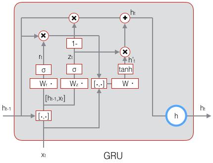
GRU的训练算法比LSTM简单一些,留给读者自行推导,本文就不再赘述了。
五、小结
至此,LSTM——也许是结构最复杂的一类神经网络——就讲完了,相信拿下前几篇文章的读者们搞定这篇文章也不在话下吧!现在我们已经了解循环神经网络和它最流行的变体——LSTM,它们都可以用来处理序列。但是,有时候仅仅拥有处理序列的能力还不够,还需要处理比序列更为复杂的结构(比如树结构),这时候就需要用到另外一类网络:递归神经网络(Recursive Neural Network),巧合的是,它的缩写也是RNN。
内容总结
以上是互联网集市为您收集整理的深度学习之长短时记忆网络(LSTM)全部内容,希望文章能够帮你解决深度学习之长短时记忆网络(LSTM)所遇到的程序开发问题。 如果觉得互联网集市技术教程内容还不错,欢迎将互联网集市网站推荐给程序员好友。
内容备注
版权声明:本文内容由互联网用户自发贡献,该文观点与技术仅代表作者本人。本站仅提供信息存储空间服务,不拥有所有权,不承担相关法律责任。如发现本站有涉嫌侵权/违法违规的内容, 请发送邮件至 gblab@vip.qq.com 举报,一经查实,本站将立刻删除。
内容手机端
扫描二维码推送至手机访问。