首页 / 算法 / 机器学习算法系列(1)逻辑回归
机器学习算法系列(1)逻辑回归
内容导读
互联网集市收集整理的这篇技术教程文章主要介绍了机器学习算法系列(1)逻辑回归,小编现在分享给大家,供广大互联网技能从业者学习和参考。文章包含10243字,纯文字阅读大概需要15分钟。
内容图文
逻辑回归")
1、逻辑回归算法原理
(1)线性回归预测函数:线性回归模型的输出值y是连续型变量,值域为R
y=Xθ
(2)sigmoid函数:
g(z)=1+e?z1?
(3)逻辑回归预测函数:逻辑回归的输出值y是离散型变量,值域为{0,1}
hθ?(X)=g(Xθ)=1+e?Xθ1?
逻辑回归模型是在线性回归模型输出值y经过sigmoid变换得到的,即通过将线性回归原本的值域映射到{0,1}区间内,当取值大于临界值(例如0.5)时为一类,小于临界值时为另一类,从而达到分类的目的。
2、逻辑回归算法实现
信用卡欺诈案例:
#导入库
import numpy as np
import pandas as pd
import matplotlib.pyplot as plt
import seaborn as sns

import warnings
warnings.filterwarnings("ignore")#忽略警告

%matplotlib inline
#读取数据
data = pd.read_csv("creditcard.csv")
pd.set_option("display.max_columns",None)#显示所有列
print("数据结构:",data.shape)
data.head()
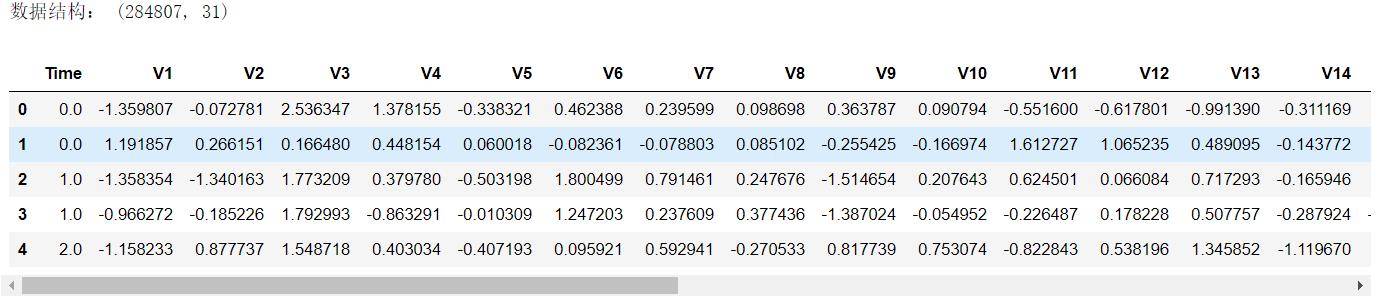
分析:贷款金额"Amount"需要做数据标准化。
#标签分布
sns.countplot( x = "Class",data = data,linewidth = 2)#seaborn可视化库中的柱状图
plt.title("Fraud class histogram")
plt.xlabel("Class")
plt.ylabel("Frequency")
plt.show()
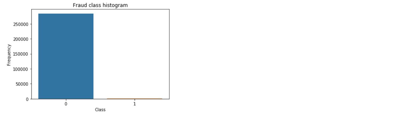
分析:正负例样本数相差较大,需要使用下采样或者过采样处理数据。
2.1、数据预处理
2.1.1 数据标准化
from sklearn.preprocessing import StandardScaler
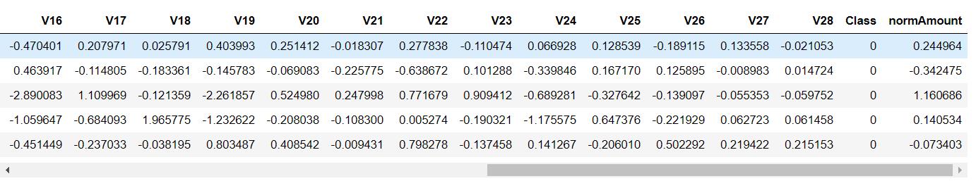
data["normAmount"] = StandardScaler().fit_transform(data["Amount"].values.reshape(-1,1))#数据标准化
data2 = data.drop(["Time","Amount"],axis = 1)#删除列
data2.head()
2.2、挖掘建模
2.2.1 下采样方案
(1)数据下采样
X = data2.ix[:,data2.columns != "Class"]#取特征值
y = data2.ix[:,data2.columns == "Class"]#取标签值

number_records_fraud = len(data2[data2.Class == 1])#欺诈样本数量

fraud_indices = np.array(data2[data2.Class == 1].index)#欺诈样本索引
normal_indices = data2[data2.Class == 0].index#正常样本索引

random_normal_indices = np.random.choice(normal_indices,number_records_fraud,replace = False)#随机选择和异常样本数量一致的正常样本
random_normal_indices = np.array(random_normal_indices)#下采样正常样本索引

under_sample_indices = np.concatenate([fraud_indices,random_normal_indices])#数据合并

under_sample_data = data2.iloc[under_sample_indices,:]#下采样样本
X_under_sample = under_sample_data.ix[:,under_sample_data.columns != "Class"]#下采样样本特征
y_under_sample = under_sample_data.ix[:,under_sample_data.columns == "Class"]#下采样样本标签

print("正常样本比例:",len(under_sample_data[under_sample_data.Class == 0])/len(under_sample_data))
print("异常样本比例:",len(under_sample_data[under_sample_data.Class == 1])/len(under_sample_data))
print("下采样总体样本数量:",len(under_sample_data))
索引使用参考:https://blog.csdn.net/qq1483661204/article/details/77587881

(2)数据集划分
from sklearn.model_selection import train_test_split
X_train,X_test,y_train,y_test = train_test_split(X,y,test_size = 0.3,random_state = 0)
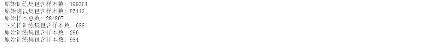
print("原始训练集包含样本数:",X_train.shape[0])
print("原始测试集包含样本数:",X_test.shape[0])
print("原始样本总数:",X.shape[0])
X_train_undersample,X_test_undersample,y_train_undersample,y_test_undersample = train_test_split(X_under_sample,y_under_sample,test_size = 0.3,random_state = 0)
print("下采样训练集包含样本数:",X_train_undersample.shape[0])
print("原始训练集包含样本数:",X_test_undersample.shape[0])
print("原始训练集包含样本数:",under_sample_data.shape[0])
(3)评估标准:召回率
* Recall = TP/(TP+FN)
* 召回率 = 正确判断异常样本/所有异常样本
(4)基础模型
#导入库
from sklearn.model_selection import GridSearchCV
from sklearn.linear_model import LogisticRegression
from sklearn.model_selection import KFold, cross_val_score
from sklearn.metrics import confusion_matrix,recall_score,classification_report
#基础模型构建
lr = LogisticRegression(C = 0.1, penalty = "l1",solver = "liblinear")
lr.fit(X_train_undersample,y_train_undersample)
y_pred_undersample = lr.predict(X_test_undersample)
print("Recall Score:",recall_score(y_test_undersample,y_pred_undersample))

(5)调参(正则化惩罚项)
逻辑回归Sklearn参数:
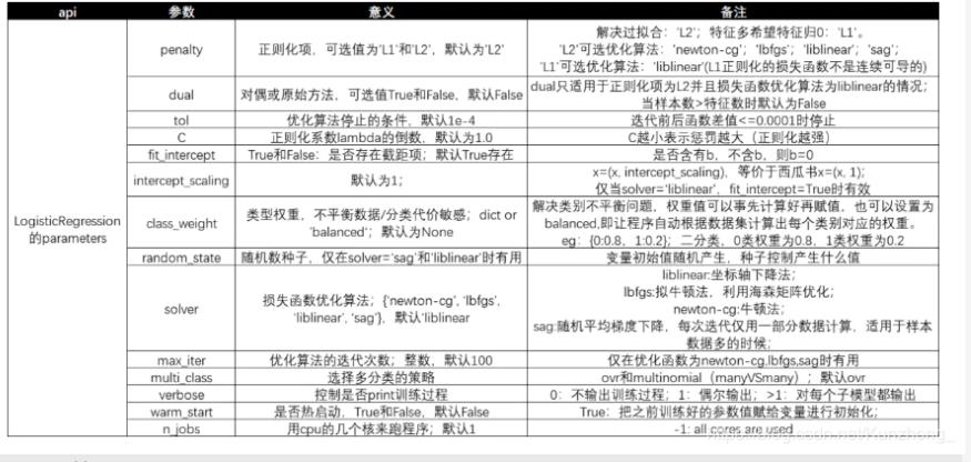
分析:需要调的参数只有C、阈值。
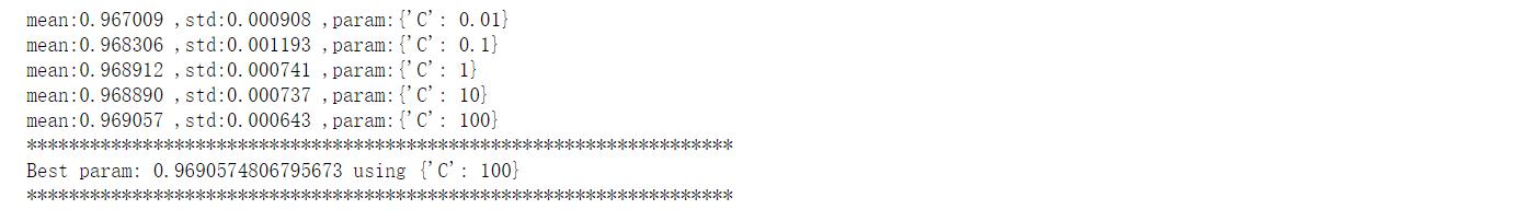
#正则化惩罚项调参
parameters = {'C':[0.01,0.1,1,10,100]}
%%time

grid = GridSearchCV(lr,param_grid = parameters,scoring = "recall",cv = 5)
grid.fit(X_train_undersample,y_train_undersample)
means = grid.cv_results_['mean_test_score']
stds = grid.cv_results_['std_test_score']
params = grid.cv_results_['params']

for mean,std,param in zip(means,stds,params):
    print("mean:%f ,std:%f ,param:%r" % (mean,std,param))
print("*******************************************************************")
print('Best param: {} using {}'.format(grid.best_score_, grid.best_params_))
print("*******************************************************************")
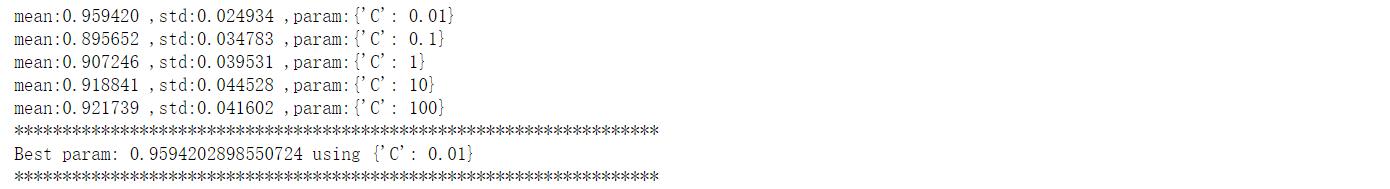
分析:调参三步走(1)需要调的参数写成字典的形式;(2)网格搜索,交叉验证;(3)输出结果
(6)混淆矩阵
下采样样本混淆矩阵:
#混淆矩阵模板,使用时传入参数即可
def plot_confusion_matrix(cm,classes,title = "Confusion matrix",cmap = plt.cm.Blues):
    plt.imshow(cm,interpolation = "nearest",cmap = cmap)
    plt.title(title)
    plt.colorbar()
    tick_marks = np.arange(len(classes))
    plt.xticks(tick_marks,classes,rotation = 0)
    plt.yticks(tick_marks,classes)

    thresh = cm.max()/2
    for i, j in itertools.product(range(cm.shape[0]), range(cm.shape[1])):
        plt.text(j, i, cm[i, j],horizontalalignment="center",color="white" if cm[i, j] > thresh else "black")

    plt.tight_layout()
    plt.ylabel("True label")
    plt.xlabel("Predicted label")
import itertools
lr = LogisticRegression(C = 0.01, penalty = "l1",solver = "liblinear")
lr.fit(X_train_undersample,y_train_undersample)
y_pred_undersample = lr.predict(X_test_undersample)

# Compute confusion matrix
cnf_matrix = confusion_matrix(y_test_undersample,y_pred_undersample)
np.set_printoptions(precision = 2)

print("Recall metric in the testing dataset: ", cnf_matrix[1,1]/(cnf_matrix[1,0] + cnf_matrix[1,1]))

# Plot non-normalized confusion matrix
class_names = [0,1]
plt.figure()
plot_confusion_matrix(cnf_matrix,classes=class_names,title="Confusion matrix")
plt.show()

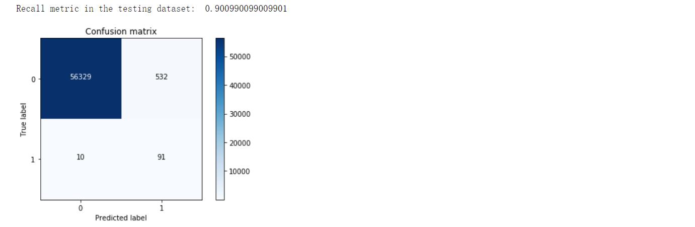
全样本混淆矩阵:
lr = LogisticRegression(C = 0.01, penalty = "l1",solver = "liblinear")
lr.fit(X_train_undersample,y_train_undersample)
y_pred = lr.predict(X_test)

# Compute confusion matrix
cnf_matrix = confusion_matrix(y_test,y_pred)
np.set_printoptions(precision = 2)

print("Recall metric in the testing dataset: ", cnf_matrix[1,1]/(cnf_matrix[1,0] + cnf_matrix[1,1]))

# Plot non-normalized confusion matrix
class_names = [0,1]
plt.figure()
plot_confusion_matrix(cnf_matrix,classes=class_names,title="Confusion matrix")
plt.show()
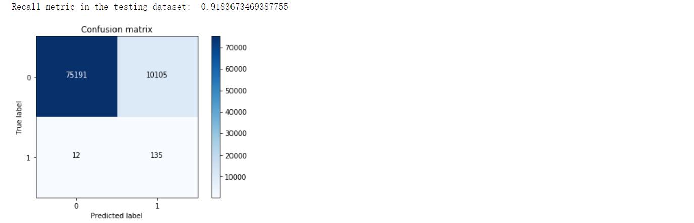
分析:右上角FP=10105,本来为负例被判断为正例的样本,统计学上第二类错误,“纳伪”,左下角TN=12,本来为正例被判断为负例的样本,统计学上第一类错误,“弃真”。可见,相对于下采样样本,全样本的Recall值略微下降,但FP大幅度增加,说明下采样方法存在一定缺陷。
混淆矩阵参考:https://blog.csdn.net/Orange_Spotty_Cat/article/details/80520839
(7)调参(阈值)
lr = LogisticRegression(C = 0.01, penalty = "l1",solver = "liblinear")
lr.fit(X_train_undersample,y_train_undersample.values.ravel())
y_pred_undersample = lr.predict_proba(X_test_undersample.values)

thresholds = [0.1,0.2,0.3,0.4,0.5,0.6,0.7,0.8,0.9]
plt.figure(figsize = (10,10))
j = 1
for i in thresholds:
    y_test_predictions_high_recall = y_pred_undersample[:,1] > i

    plt.subplot(3,3,j)
    j += 1
    cnf_matrix = confusion_matrix(y_test_undersample,y_test_predictions_high_recall)
    np.set_printoptions(precision = 2)
    print("给定阈值:",i,"时测试集召回率",cnf_matrix[1,1]/(cnf_matrix[1,0] + cnf_matrix[1,1]))
    class_names = [0,1]
    plot_confusion_matrix(cnf_matrix,classes = class_names,title ="Threshold >= %s"%i)
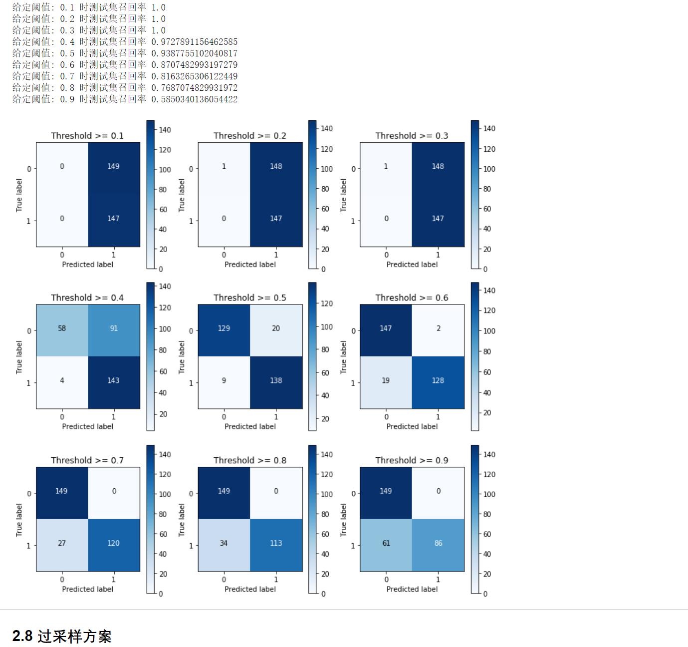
2.2.2 过采样方案
#导入库
import pandas as pd
from imblearn.over_sampling import SMOTE
from sklearn.ensemble import RandomForestClassifier
from sklearn.metrics import confusion_matrix
from sklearn.model_selection import train_test_split
#导入数据
credit_cards = pd.read_csv("creditcard.csv")

columns = credit_cards.columns
# The labels are in the last column ("Class"). Simply remove it to obtain features columns
features_columns = columns.delete(len(columns)-1)

features = credit_cards[features_columns]
labels = credit_cards["Class"]
#数据集划分
features_train, features_test, labels_train, labels_test = train_test_split(features,labels,test_size = 0.2,random_state = 0)
#使用SMOTE进行过采样
oversampler = SMOTE(random_state = 0)
os_features,os_labels = oversampler.fit_sample(features_train,labels_train)#基于SMOTE算法进行样本生成,正例、负例一样多
len(os_labels[os_labels == 1])

#转换格式
os_features = pd.DataFrame(os_features)
os_labels = pd.DataFrame(os_labels)
#调参
%%time

grid = GridSearchCV(lr,param_grid = parameters,scoring = "recall",cv = 5)
grid.fit(os_features,os_labels)
#输出调参结果
means = grid.cv_results_['mean_test_score']
stds = grid.cv_results_['std_test_score']
params = grid.cv_results_['params']

for mean,std,param in zip(means,stds,params):
    print("mean:%f ,std:%f ,param:%r" % (mean,std,param))
print("*******************************************************************")
print('Best param: {} using {}'.format(grid.best_score_, grid.best_params_))
print("*******************************************************************")
#画出混淆矩阵
lr = LogisticRegression(C = 100, penalty = 'l1',solver = "liblinear")
lr.fit(os_features,os_labels.values.ravel())
y_pred = lr.predict(features_test.values)

# Compute confusion matrix
cnf_matrix = confusion_matrix(labels_test,y_pred)
np.set_printoptions(precision = 2)

print("Recall metric in the testing dataset: ", cnf_matrix[1,1]/(cnf_matrix[1,0] + cnf_matrix[1,1]))

# Plot non-normalized confusion matrix
class_names = [0,1]
plt.figure()
plot_confusion_matrix(cnf_matrix,classes=class_names,title = "Confusion matrix")
plt.show()
分析:过采样方法Rcall值有所降低,但是TN大幅度减少。
三、逻辑回归总结
主要知识点:
(1)数据标准化
(2)数据采样方法
(3)逻辑回归调参
(4)混淆矩阵
逻辑回归优缺点:
优点:
(1)预测结果是界于0和1之间的概率;
(2)可以适用于连续性和类别性自变量;
(3)容易使用和解释;
缺点:
(1)对模型中自变量多重共线性较为敏感,例如两个高度相关自变量同时放入模型,可能导致较弱的一个自变量回归符号不符合预期,符号被扭转。?需要利用因子分析或者变量聚类分析等手段来选择代表性的自变量,以减少候选变量之间的相关性;
(2)预测结果呈“S”型,因此从log(odds)向概率转化的过程是非线性的,在两端随着?log(odds)值的变化,概率变化很小,边际值太小,slope太小,而中间概率的变化很大,很敏感。 导致很多区间的变量变化对目标概率的影响没有区分度,无法确定阀值。
内容总结
以上是互联网集市为您收集整理的机器学习算法系列(1)逻辑回归全部内容,希望文章能够帮你解决机器学习算法系列(1)逻辑回归所遇到的程序开发问题。 如果觉得互联网集市技术教程内容还不错,欢迎将互联网集市网站推荐给程序员好友。
内容备注
版权声明:本文内容由互联网用户自发贡献,该文观点与技术仅代表作者本人。本站仅提供信息存储空间服务,不拥有所有权,不承担相关法律责任。如发现本站有涉嫌侵权/违法违规的内容, 请发送邮件至 gblab@vip.qq.com 举报,一经查实,本站将立刻删除。
内容手机端
扫描二维码推送至手机访问。